backscatterBicyclist

Backscatter radar signals from bicyclist

Since R2021a

Description

The backscatterBicyclist object simulates backscattered radar signals reflected from a moving bicyclist. The bicyclist consists of both the bicycle and its rider. The object models the motion of the bicyclist and computes the sum of all reflected signals from multiple discrete scatterers on the bicyclist. The model ignores internal occlusions within the bicyclist. The reflected signals are based on a multi-scatterer model developed from a 77 GHz radar system.

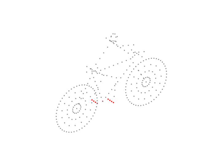
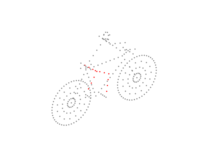
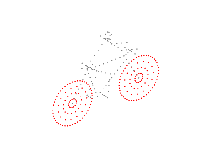
Scatterers are located on five major bicyclist components:

• Bicycle frame and rider

• Bicycle pedals

• Upper and lower legs of the rider

• Front wheel

• Back wheel

Excluding the wheels, there are 114 scatterers on the bicyclist. The wheels contain scatterers on the rim and spokes. The number of scatterers on the wheels depends on the number of spokes per wheel. The number of spokes is specified using the NumWheelSpokes property.

You can obtain the current bicyclist position and velocity by calling the move object function. Calling this function also updates the position and velocity for the next time epoch. To obtain the reflected signal, call the reflect object function. You can plot the instantaneous position of the bicyclist using the plot object function.

Creation

Syntax

bicyclist = backscatterBicyclist
bicyclist = backscatterBicyclist(Name,Value,...)


Description

bicyclist = backscatterBicyclist creates a backscatterBicyclist object, bicyclist, having default property values.

bicyclist = backscatterBicyclist(Name,Value,...) creates a backscatterBicyclist object, bicyclist, with each specified property Name set to the specified Value. You can specify additional name-value pair arguments in any order as (Name1,Value1,...,NameN,ValueN). Any unspecified properties take default values. For example,

bicyclist = backscatterBicyclist( ...
              'NumWheelSpokes',18,'Speed',10.0, ...
              'InitialPosition',[0;0;0],'InitialHeading',90, ...
              'GearTransmissionRatio',5.5);

models a bicycle with 18 spokes on each wheel that is moving along the positive y-axis at 10 meters per second. The gear transmission ratio of 5.5 indicates that there are 5.5 wheel rotations for each pedal rotation. The bicyclist is heading along the y-axis.

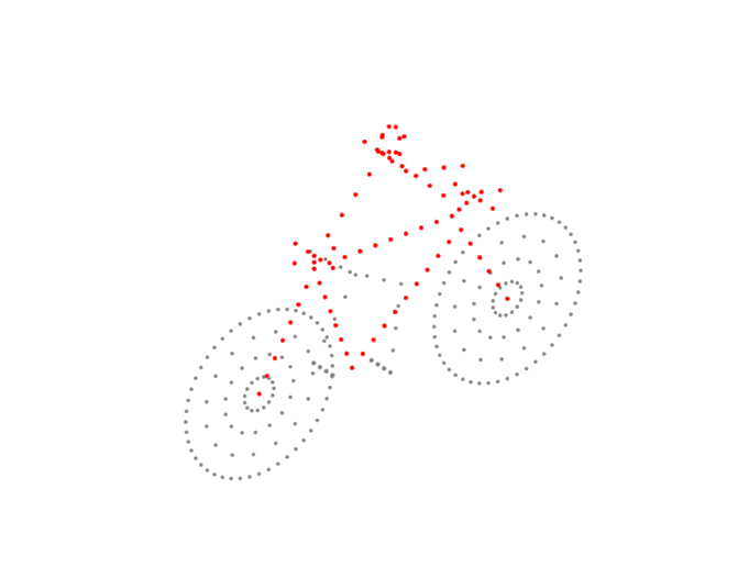
This figure illustrates a bicyclist starting to turn left.

Properties

NumWheelSpokes — Number of spokes per wheel

20 (default) | positive integer

Number of spokes per wheel of the bicycle, specified as a positive integer from 3 to 50, inclusive.

Data Types: double

GearTransmissionRatio — Ratio of wheel rotations to pedal rotations

1.5 (default) | positive scalar

Ratio of wheel rotations to pedal rotations, specified as a positive scalar. The gear ratio must be in the range from 0.5 through 6. Units are dimensionless.

Data Types: double

OperatingFrequency — Carrier frequency of narrowband signals

77e9 (default) | positive scalar

Carrier frequency of the narrowband incident signals, specified as a positive scalar. Units are in Hz.

Example: 900e6

Data Types: double

InitialPosition — Initial position of bicyclist

[0;0;0] (default) | 3-by-1 real-valued vector

Initial position of the bicyclist, specified as a 3-by-1 real-valued vector in the form of [x;y;z] in global coordinates. Units are in meters. The initial position corresponds to the location of the origin of the bicycle coordinates. The origin is at the center of mass of the scatterers of the default bicyclist configuration projected onto the ground.

Data Types: double

InitialHeading — Initial heading of bicyclist

0 (default) | scalar

Initial heading of bicyclist, specified as a scalar. Heading is measured in the xy-plane from the x-axis towards the y-axis. Heading is with respect to global coordinates. Units are in degrees.

Data Types: double

Speed — Speed of bicyclist

4 (default) | nonnegative scalar

Speed of bicyclist, specified as a nonnegative scalar. The motion model limits the speed to a maximum of 60 m/s (216 kph). Speed is defined with respect to global coordinates. Units are in meters per second.

Data Types: double

Coast — Set bicycle coasting state

false (default) | true

Set bicycle coasting state, specified as false or true. If set to true, the bicyclist is not pedaling, but the wheels are still rotating (freewheeling). If set to false, the bicyclist is pedaling, and the GearTransmissionRatio determines the wheel rotations to pedal rotations.

Data Types: logical

PropagationSpeed — Signal propagation speed (m/s)

physconst('LightSpeed') (default) | positive scalar

Signal propagation speed, specified as a positive scalar. Units are in meters per second (m/s). The default propagation speed is the value returned by physconst('LightSpeed'). See physconst for more information.

Example: 3e8

Data Types: double

AzimuthAngles — Radar cross-section azimuth angles

[-180:180] (default) | 1-by-P real-valued row vector | P-by-1 real-valued column vector

Radar cross-section azimuth angles, specified as a 1-by-P or P-by-1 real-valued vector. This property defines the azimuth coordinates of each column of the radar cross-section matrix specified by the RCSPattern property. P must be greater than two. Angle units are in degrees.

Example: [-45:0.1:45]

Data Types: double

ElevationAngles — Radar cross-section elevation angles

0 (default) | scalar | 1-by-Q real-valued row vector | Q-by-1 real-valued column vector

Radar cross-section elevation angles, specified as a 1-by-Q or Q-by-1 real-valued vector. This property defines the elevation coordinates of each row of the radar cross-section matrix specified by the RCSPattern property. Q must be greater than two. Angle units are in degrees.

Example: [-30:0.1:30]

Data Types: double

RCSPattern — Radar cross-section pattern

1-by-361 real-valued matrix (default) | Q-by-P real-valued vector | 1-by-P real-valued vector

Radar cross-section (RCS) pattern, specified as a Q-by-P real-valued matrix or a 1-by-P real-valued vector. Matrix rows represent constant elevation, and columns represent constant azimuth. Q is the length of the vector defined by the ElevationAngles property. P is the length of the vector defined by the AzimuthAngles property. Units are in square meters.

You can also specify the pattern as a 1-by-P real-valued vector of azimuth angles for a single elevation.

The default value of this property is a 1-by-361 matrix containing values derived from 77 GHz radar measurements of a bicyclist. The default values of AzimuthAngles and ElevationAngles correspond to the default RCS matrix.

Example: [1,.5;.5,1]

Data Types: double

Object Functions

Specific to This Object

getNumScatterers	Number of scatterers on bicyclist
move	Position, velocity, and orientation of moving bicyclist
plot	Display locations of scatterers on bicyclist
reflect	Reflected signal from moving bicyclist

Common to All System Objects

step	Run System object algorithm
release	Release resources and allow changes to System object property values and input characteristics
reset	Reset internal states of System object

Examples

Radar Signal Backscattered by Bicyclist

Compute the backscattered radar signal from a bicyclist moving along the x-axis at 5 m/s away from a radar. Assume that the radar is located at the origin. The radar transmits an LFM signal at 24 GHz with a 300 MHz bandwidth. A signal is reflected at the moment the bicyclist starts to move and then one second later.

Initialize Bicyclist, Waveform, and Propagation Channel Objects

Initialize the backscatterBicyclist, phased.LinearFMWaveform, and phased.FreeSpace objects. Assume a 300 MHz sampling frequency. The initial position of the bicyclist lies on the x-axis 30 meters from the radar.

bw = 300e6;
fs = bw;
fc = 24e9;
radarpos = [0;0;0];
bpos = [30;0;0];
bicyclist = backscatterBicyclist( ...
    'OperatingFrequency',fc,'NumWheelSpokes',15, ...
    'InitialPosition',bpos,'Speed',5.0, ...
    'InitialHeading',0.0);
lfmwav = phased.LinearFMWaveform( ...
    'SampleRate',fs, ...
    'SweepBandwidth',bw);
sig = lfmwav();
chan = phased.FreeSpace( ...
    'OperatingFrequency',fc, ...
    'SampleRate',fs, ...
    'TwoWayPropagation',true);

Plot Initial Bicyclist Position

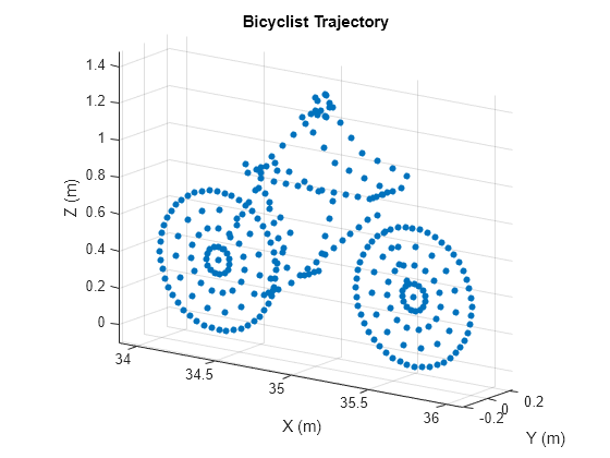
Using the move object function, obtain the initial scatterer positions, velocities and the orientation of the bicyclist. Plot the initial position of the bicyclist. The dt argument of the move object function determines that the next call to move returns the bicyclist state of motion dt seconds later.

dt = 1.0;
[bpos,bvel,bax] = move(bicyclist,dt,0);
plot(bicyclist)

Obtain First Reflected Signal

Propagate the signal to all scatterers and obtain the cumulative reflected return signal.

N = getNumScatterers(bicyclist);
sigtrns = chan(repmat(sig,1,N),radarpos,bpos,[0;0;0],bvel);
[rngs,ang] = rangeangle(radarpos,bpos,bax);
y0 = reflect(bicyclist,sigtrns,ang);

Plot Bicyclist Position After Position Update

After the bicyclist has moved, obtain the scatterer positions and velocities and then move the bicycle along its trajectory for another second.

[bpos,bvel,bax] = move(bicyclist,dt,0);
plot(bicyclist)

Obtain Second Reflected Signal

Propagate the signal to all scatterers at their new positions and obtain the cumulative reflected return signal.

sigtrns = chan(repmat(sig,1,N),radarpos,bpos,[0;0;0],bvel);
[~,ang] = rangeangle(radarpos,bpos,bax);
y1 = reflect(bicyclist,sigtrns,ang);

Match Filter Reflected Signals

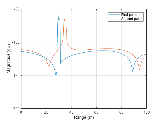
Match filter the reflected signals and plot them together.

mfsig = getMatchedFilter(lfmwav);
nsamp = length(mfsig);
mf = phased.MatchedFilter('Coefficients',mfsig);
ymf = mf([y0 y1]);
fdelay = (nsamp-1)/fs;
t = (0:size(ymf,1)-1)/fs - fdelay;
c = physconst('LightSpeed');
plot(c*t/2,mag2db(abs(ymf)))
ylim([-200 -50])
xlabel('Range (m)')
ylabel('Magnitude (dB)')
ax = axis;
axis([0,100,ax(3),ax(4)])
grid
legend('First pulse','Second pulse')

Compute the difference in range between the maxima of the two pulses.

[maxy,idx] = max(abs(ymf));
dpeaks = t(1,idx(2)) - t(1,idx(1));
drng = c*dpeaks/2

drng = 
4.9965

The range difference is 5 m, as expected given the bicyclist speed.

Display Micro-Doppler Shift from Moving Bicyclist

Display a spectrogram showing the micro-Doppler effect on radar signals reflected from the scatterers on a moving bicyclist target. A stationary radar transmits 1000 pulses of an FMCW radar wave with a bandwidth of 250 MHz and of 1 $\mu \sec$duration. The radar operates at 24 GHz. The bicyclist starts 5 m from the radar and moves away at 4 m/s.

Set up the waveform, channel, transmitter, receiver, and platform System objects.

bw = 250e6;
fs = 2*bw;
fc = 24e9;
c = physconst('Lightspeed');
tm = 1e-6;
wav = phased.FMCWWaveform('SampleRate',fs,'SweepTime',tm, ...
    'SweepBandwidth',bw);
chan = phased.FreeSpace('PropagationSpeed',c,'OperatingFrequency',fc, ...
    'TwoWayPropagation',true,'SampleRate',fs);
radarplt = phased.Platform('InitialPosition',[0;0;0], ...
    'OrientationAxesOutputPort',true);
trx = phased.Transmitter('PeakPower',1,'Gain',25);
rcvx = phased.ReceiverPreamp('Gain',25,'NoiseFigure',10);

Create a bicyclist object moving at 4 meters/second.

bicyclistSpeed = 4;
bicyclist = backscatterBicyclist('InitialPosition',[5;0;0],'Speed',bicyclistSpeed, ...
    'PropagationSpeed',c,'OperatingFrequency',fc,'InitialHeading',0.0);
lambda = c/fc;
fmax = 2*bicyclist.GearTransmissionRatio*bicyclistSpeed/lambda;
tsamp = 1/(2*fmax);

Loop over 1000 pulses. Find the angle of incidence of the radar. Propagate the wave to each scatterer, and then reflect the wave from the scatterers back to the radar.

npulse = 1000;
xr = complex(zeros(round(fs*tm),npulse));
for m = 1:npulse
    [posr,velr,axr] = radarplt(tsamp);
    [post,velt,axt] = move(bicyclist,tsamp,0);
    [~,angrt] = rangeangle(posr,post,axt);
    x = trx(wav());
    xt = chan(repmat(x,1,size(post,2)),posr,post,velr,velt);
    xr(:,m) = rcvx(reflect(bicyclist,xt,angrt));
end

Process the arriving signals. First, dechirp the signal and then pass the signal into a Kaiser-windowed short-time Fourier transform.

xd = conj(dechirp(xr,x));
M = 128;
beta = 6;
w = kaiser(M,beta);
R = floor(1.7*(M-1)/(beta+1));
noverlap = M - R;
[S,F,T] = stft(sum(xd),1/tsamp,'Window',w,'FFTLength',M*2, ...
    'OverlapLength',noverlap);
maxval = max(10*log10(abs(S)));
pcolor(T,-F*lambda/2,10*log10(abs(S))-maxval);
shading flat;
colorbar
xlabel('Time (sec)')
ylabel('Speed (m/s)')

Backscatter Bicyclist With Custom RCS Pattern

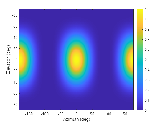
Create a custom RCS pattern to use with the backscatterBicyclist object.

The RCS pattern is computed from cosines raised to the fourth power. Plot the pattern.

az = [-180:180];
el = [-90:90];
caz = cosd(az').^4;
cel = cosd(el).^4;
rcs = (caz*cel)';
imagesc(az,el,rcs)
xlabel('Azimuth (deg)')
ylabel('Elevation (deg)')
colorbar

bicyclist = backscatterBicyclist( ...
    'NumWheelSpokes',18,'Speed',10.0, ...
    'InitialPosition',[0;0;0],'InitialHeading',90, ...
    'GearTransmissionRatio',5.5,'AzimuthAngles',az, ...
    'ElevationAngles',el,'RCSPattern',rcs);

Algorithms

Bicycle Model

The bicyclist consists of five primary components: bicycle frame and rider, pedals, rider legs, front wheel, and rear wheel. Each component contains many scatterers. All components move with a velocity determined by the specified speed and heading properties. In addition, the legs, pedals, and wheels undergo cyclical motion determined by the speed.

Motion of Scatterers on Frame and Rider

Scatterers on the frame and rider are fixed with respect to the bicyclist and move with the ego velocity

$${\overrightarrow{\upsilon }}_{\text{ego}}=\upsilon \cos H\widehat{i}+\upsilon \sin H\widehat{j}$$

where v is the speed of the bicyclist specified by the Speed property and H is the heading specified by the InitialHeading property. These properties can be changed by calling the move function.

This figure shows the location of the scatterers on the bicycle frame and rider.

Motion of Scatterers on Pedals

Scatterers on the pedals move with the bicyclist but can also revolve around the crank spindle with a radius of rotation R_ped. There are two possible motions of the pedals depending upon whether the bicycle is coasting (freewheeling) or not coasting:

• When the bicycle is coasting, the pedals do not revolve around the crank spindle and the velocity of the pedal scatterers equals the bicyclist velocity. Their positions relative to the bicyclist are fixed. Coasting is turned on by setting the Coast property to true or by setting the coast argument of the move object function to true. The speed of the pedal is

  $${\overrightarrow{\upsilon }}_{\text{ped,tot}}={\overrightarrow{\upsilon }}_{\text{ego}}$$

• When the bicycle is not coasting, the rider is pedaling. The angular velocity of the pedals is related to the angular velocity of the wheels by

  $${\overrightarrow{\omega }}_{\text{wh}}=G{\overrightarrow{\omega }}_{\text{ped}}$$

  where G is the gear ratio defined by the GearTransmissionRatio property. The speed of a pedal scatterer equals the rotational speed of the pedal multiplied by the distance from pedal to crank spindle. The vector form of this relationship is:

  $${\overrightarrow{\upsilon }}_{\text{ped}}={\overrightarrow{\omega }}_{\text{ped}}\times {\overrightarrow{r}}_{\text{ped}}$$

  The velocity of the pedal with respect to the bicyclist is then

  $${\overrightarrow{\upsilon }}_{\text{ped,tot}}={\overrightarrow{\omega }}_{\text{ped}}\times {\overrightarrow{r}}_{\text{ped}}+{\overrightarrow{\upsilon }}_{\text{ego}}=G{\overrightarrow{\omega }}_{\text{wh}}\times {\overrightarrow{r}}_{\text{ped}}+{\overrightarrow{\upsilon }}_{\text{ego}}$$

  Coasting is turned off by setting the Coast property to false or by setting the coast argument of the move object function to false.

This figure shows the locations of the pedal scatterers.

Motion of Scatterers on Riders Legs

Scatterers on the upper and lower legs of the rider move with the bicycle with an added cyclical motion. There are two possible motions of the legs depending upon whether the bicycle is coasting or not coasting:

• When the bicycle is coasting, the legs are not moving with the respect to the bicycle and the scatterers move with the velocity of the bicyclist. Coasting is turned on by setting the Coast property to true or by setting the coast argument of the move object function to true.

• When the bicycle is not coasting, the upper and lower legs execute reciprocating motion. The upper legs partially rotate around the hip of the rider. The foot is attached to the pedal and rotates with the pedal. The knee connects the lower and upper legs. The locations of the foot and hips of the rider determine the locations of the knees and the motion of the scatterers on the legs.

  Coasting is turned off by setting the Coast property to false or by setting the coast argument of the move object function to false.

This figure shows the locations of the scatterers on the upper and lower legs of the rider.

Motion of Scatterers on Bicycle Wheels

Scatterers are on the spokes and rims of the wheels and revolve around the wheel axle at varying distances, r_spk, from the axle. The velocity of the scatterers in the bicyclist frame of reference is

$${\overrightarrow{\upsilon }}_{\text{spk}}={\overrightarrow{\omega }}_{\text{wh}}\times {\overrightarrow{r}}_{\text{spk}}$$

The absolute velocity of a spoke or rim scatterer is

$${\overrightarrow{\upsilon }}_{\text{spk}}={\overrightarrow{\omega }}_{\text{wh}}\times {\overrightarrow{r}}_{\text{spk}}+{\overrightarrow{\upsilon }}_{\text{ego}}$$

This figure shows the locations of the scatterers on the wheel rims and spokes.

Radar Cross-Section

The value of the radar cross-section (RCS) of a scatterer generally depends upon the incident angle of the reflected radiation. The backscatterBicyclist object uses a simplified RCS model: the RCS pattern of an individual scatterer equals the total bicyclist pattern divided by the number of scatterers. The value of the RCS is computed from the RCS pattern evaluated at an average over all scatterers of the azimuth and elevation incident angles. Therefore, the RCS value is the same for all scatterers. You can specify the RCS pattern using the RCSPattern property of the backscatterBicyclist object or use the default value.

References

[1] Stolz, M. et al. "Multi-Target Reflection Point Model of Cyclists for Automotive Radar." 2017 European Radar Conference (EURAD), Nuremberg, 2017, pp. 94–97.

[2] Chen, V., D. Tahmoush, and W. J. Miceli. Radar Micro-Doppler Signatures: Processing and Applications. The Institution of Engineering and Technology: London, 2014.

[3] Belgiovane, D., and C. C. Chen. "Bicycles and Human Rider Backscattering at 77 GHz for Automotive Radar." 2016 10^th European Conference on Antennas and Propagation (EuCAP), Davos, 2016, pp. 1–5.

[4] Victor Chen, The Micro-Doppler Effect in Radar. Norwood, MA: Artech House, 2011.

Extended Capabilities

C/C++ Code Generation
Generate C and C++ code using MATLAB® Coder™.

Version History

Introduced in R2021a