Record Raw ADC Data for Offline Processing from TI mmWave Radar Board Using DCA1000EVM Capture Card
R2026bThis example shows how to use Radar Toolbox Support Package for Texas Instruments® mmWave Radar Sensors to read and record raw ADC radar data (IQ data) from Texas Instruments (TI) radars in binary files and analyze the recorded data.
This example evaluates and visualizes the range response and range-doppler response using the ADC data recorded from the TI mmWave radar.
This example supports boards operating in both TDM (Time Division Multiplexing) and DDM (Doppler Division Multiplexing) modes.
Required Products
MATLAB®
Radar Toolbox Support Package for Texas Instruments mmWave Radar Sensors
For information on installing the support package, see Install Support and Perform Hardware Setup for TI mmWave Hardware.
Required Hardware
One of the supported TI mmWave Radar Evaluation Modules (EVM) that supports reading raw ADC data (IQ data) by connecting to DCA1000EVM (see Supported Boards)
USB Cable Type A to Micro B
Power Adaptor: Either 5V, 3 A power adapter (for AWR1642BOOST, IWR1642BOOST, AWR1843BOOST) or 12V, 2.5A power adapter (for AWR2944EVM). In both cases, it is recommended that you connect two power adapters of the same kind to the two independent power input connectors in these boards.
DCA1000EVM capture card
Samtec cable
Ethernet cable
Hardware Setup
You must set up the TI mmWave radar sensor before you can use it to read ADC data to MATLAB. Set up the sensor by completing the hardware setup procedure (as explained in the Hardware Setup screens). To launch hardware setup, execute the below command and follow the steps shown in the screens.
mmWaveRadarSetup
For information on launching the Hardware Setup screens, see Install Support and Perform Hardware Setup for TI mmWave Hardware.
Connect to mmWave Radar and DCA1000 Capture card
After the hardware setup process is completed successfully, you can connect to the TI Radar board and DCA1000 by specifying the board name. This example uses the IWR6843ISK EVM. If you are using a different EVM, change the board name accordingly.
dca = dca1000("IWR6843ISK");If you have connected only one TI Radar board to the host computer, MATLAB detects the serial port details automatically. If you have connected more than one board or if MATLAB does not automatically populate the serial port details, specify the ConfigPort argument. For example:
dca = dca1000("IWR6843ISK",ConfigPort = "COM3")
Refer to Identifying Serial Ports for TI mmWave Radar Connection to identify the Config port corresponding to your board.
Note: If you are using AWR2944EVM, the board supports both TDM and DDM processing modes. The active processing mode depends on the firmware image flashed to the board during hardware setup (mmWaveRadarSetup).
DDM firmware enables all TX antennas to transmit simultaneously using Doppler-division phase coding
TDM firmware enables TX antennas to transmit sequentially in a round-robin pattern
To ensure correct operation of AWR2944EVM, use a configuration file and processing workflow that match the firmware flashed on the board. All other supported boards use TDM processing only.
dca = dca1000("AWR2944EVM")
Configuring the TI Radar
To configure the TI mmWave radar board, you must send a sequence of commands to the board using the serial port. The sequence includes commands specifying the chirp profile, sampling rate, and so on. Use the ConfigFile property of the dca1000 object to send the sequence of commands to the board. For more information, see Configure Radar Using a Configuration (.cfg) File for Reading Raw ADC (IQ) Data.
In this example, we will be using a default configuration that ships with support package.
Record ADC data, compute and visualize range response and range doppler response for the recorded data
This section is divided into two parts:
1. Record the ADC data from TI Radar board using DCA1000EVM capture card
2. Read radar data cubes from the recorded files, and compute and visualize range response and range doppler response for the data
Record the ADC data from TI Radar board using DCA1000EVM capture card
The properties of dca1000 object can be used to set recording parameters (Duration, location of recording, and so on). The function startRecording of dca1000 object can be used to read and record the ADC data from the TI Radar board in binary format along with other metadata in the record location specified.
The below script reads and stores ADC data from the TI Radar board for 100 seconds in the recordLocation specified.
Note: When you start the recording using the startRecording function, a pop-up window appears. Do not close this window while the recording is in progress. The window will close automatically when the recording is stopped.
clear dca
% Create connection to the TI Radar board and DCA1000EVM Capture card
dca = dca1000("IWR6843ISK");
% Specify the duration to record ADC data
dca.RecordDuration = 100;
% Specify the location at which you want to store the recorded data along
% with the recording parameters
dca.RecordLocation = "C:\TIRadarADCData\dca1000Data";
% Start recording.
% The function startRecording opens a window. Ensure that you do not
% close this window. It will automatically close when the recording
% finishes.
startRecording(dca);
% The startRecording function captures data in background.
% While this is happening, you are free to utilize MATLAB for any other
% tasks you might need to perform. The following code is designed to
% prevent MATLAB from proceeding until the recording has finished.
% The isRecording() function will return true if the recording is still
% in progress. Once the recording has concluded or if it has not started,
% the function will return false.
while isRecording(dca)
end
% Remember the record location for post-processing.
% In this example, we will save the recording location in a variable.
recordLocation = dca.RecordLocation;
% Clear the dca1000 object and remove the hardware connections if required
clear dca
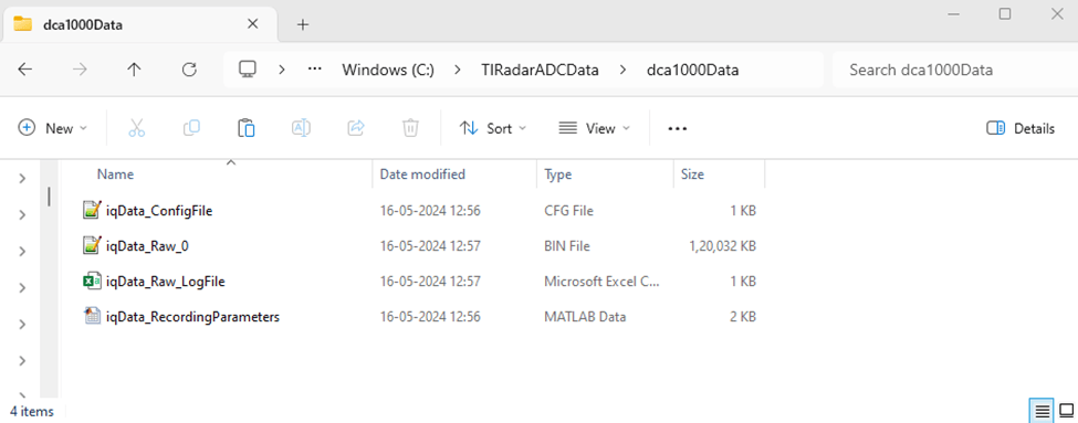
This image shows a sample of files generated along with the ADC data recordings.
Rather than setting a fixed duration for recording, you have the option to record flexibly for as long as you need. To enable this, configure the RecordDuration property of the dca1000 object to inf. When you are ready to stop recording, use the stopRecording function of the dca1000 object.
Read radar data cubes from the recorded files, and compute and visualize range response and range doppler response for the data
To read the ADC data (IQ data) cubes from these recorded binary files, you can utilize the dca1000FileReader System object. The phased.RangeResponse System object™ is used to perform range filtering on fast-time (range) data, using an FFT-based algorithm. plotResponse function of the phased.RangeResponse is used to plot the range response of the input data. The phased.RangeDopplerScope computes and displays the range-doppler response map.
% Load the recording parameters and Radar Configurations from the record
% location. This data is stored as a .mat file in the record location
temp = load(fullfile(recordLocation,'iqData_RecordingParameters.mat'));
dcaRecordingParams = temp.RecordingParameters;
% Define a variable to set the sampling rate in Hz for the
% phased.RangeResponse object. Because the dca1000 object provides the
% sampling rate in kHz, convert this rate to Hz.
fs = dcaRecordingParams.ADCSampleRate*1e3;
% Define a variable to set the FMCW sweep slope in Hz/s for the
% phased.RangeResponse object. The dca1000 object provides the
% sweep slope in MHz/us; convert this sweep slope to Hz/s.
sweepSlope = dcaRecordingParams.SweepSlope * 1e12;
% Define a variable to set the number of range samples
nr = dcaRecordingParams.SamplesPerChirp;
% Define a variable to set the center frequency in Hz for the
% phased.RangeDopplerScope object. Because the dca1000 object provides the
% center frequency in GHz, convert this rate to Hz.
fc = dcaRecordingParams.CenterFrequency*1e9;
% Chirp slow-time subsampling factor for TDM: equals the number of TX antennas.
ntx = dcaRecordingParams.NumTransmitters;
numChirpTypes = ntx;   % TDM Processing Chain
tpulse = numChirpTypes*dcaRecordingParams.ChirpCycleTime*1e-6;
% Pulse repetition frequency
prf = 1/tpulse;
% Number of active receivers
nrx = dcaRecordingParams.NumReceivers;
% Number of chirps
nchirp = dcaRecordingParams.NumChirps;
% Create phased.RangeResponse System object that performs range filtering
% on fast-time (range) data, using an FFT-based algorithm
rangeresp = phased.RangeResponse(RangeMethod = 'FFT', ...
    RangeFFTLengthSource = 'Property', ...
    RangeFFTLength = nr, ...
    SampleRate = fs, ...
    SweepSlope = sweepSlope, ...
    ReferenceRangeCentered = false);
% Create range doppler scope to compute and display the response map.
rdscope = phased.RangeDopplerScope(IQDataInput=true, ...
    SweepSlope = sweepSlope,SampleRate = fs, ...
    DopplerOutput="Speed",OperatingFrequency=fc, ...
    PRFSource="Property",PRF=prf, ...
    RangeMethod="FFT",RangeFFTLength=nr, ...
    ReferenceRangeCentered = false);
% Create a dca1000FileReader object that enables you to read ADC data (IQ data) cubes
% from the binary files recorded using the object DCA1000 in MATLAB
fr = dca1000FileReader(recordLocation = recordLocation);
% Execute the loop till all the IQ data cubes are read from the record location
while (fr.CurrentPosition <= fr.NumDataCubes)
% Read a single IQ data cube from the binary file,
% starting from the location previously accessed.
iqData = read(fr,1);
% The function read() return cell array of IQ data cube,
% extract the radar data cube from it
iqData = iqData{1};
% Get the data from first receiver antenna
iqDataRx1 = squeeze(iqData(:,1,:));
% Plots the range response corresponding to the input signal, iqData.
plotResponse(rangeresp, iqDataRx1);
% Get the data from first receiver antenna and first transmitter antenna.
% Extract every numChirpTypes-th chirp to isolate one TX phase state.
iqDataRx1Tx1 = squeeze(iqData(:,1,1:numChirpTypes:end));
% Plots the range doppler response corresponding to the the input signal.
rdscope(iqDataRx1Tx1);
end
Offline Processing of Radar Data from AWR2944EVM in DDM Mode
For the AWR2944EVM operating in Doppler Division Multiplexing (DDM) mode, offline processing uses all chirps in a frame to maximize signal-to-noise ratio (SNR) and separate the transmit (TX) channels. In contrast, the real-time processing path extracts every sixth chirp to generate a quick Range-Doppler view, which reduces processing requirements but does not preserve per-TX information. Full DDM processing performs a Doppler FFT across all chirps and then separates the TX channels by dividing the Doppler spectrum into DDM subbands.
Full DDM Processing Pipeline
The following steps describe the full DDM processing pipeline. After the Doppler FFT, the spectrum is divided into six subbands: four active subbands corresponding to the four TX antennas and two guard subbands that remain empty to maintain separation between TX responses.
Perform a Range FFT on all chirps.
Perform a Doppler FFT across all chirps in the frame.
Divide the Doppler spectrum into six subbands: four active TX subbands and two guard subbands.
Sum the power from the four active TX subbands (SumTx).
Sum the resulting power across all RX channels (SumRx).
Full DDM processing preserves the per-TX information required to form the 16-element virtual antenna array (4 TX × 4 RX). This information is essential for angle-of-arrival estimation, beamforming, and target localization.
Recording ADC data on the AWR2944EVM in DDM mode uses the same data-capture workflow as other processing modes.
Full DDM Offline Processing: Subband Extraction
The below script demonstrates the workflow of a complete DDM processing chain using recorded data cubes. The algorithm performs a Doppler FFT across all chirps in the frame, extracts the subbands associated with each TX antenna, and then combines the results across all TX and RX channels. By processing the full frame, this approach maximizes SNR while preserving the TX-channel information required for advanced radar processing.
% Load recording parameters
temp = load(fullfile(recordLocation,'iqData_RecordingParameters.mat'));
dcaParams = temp.RecordingParameters;

numADCSamples = dcaParams.SamplesPerChirp;
numRx = dcaParams.NumReceivers;
numTx = dcaParams.NumTransmitters;
numChirps = dcaParams.NumChirps;
fc = dcaParams.CenterFrequency * 1e9;            % Hz
fs = dcaParams.ADCSampleRate * 1e3;               % Hz
sweepSlope = dcaParams.SweepSlope * 1e12;         % Hz/s
rangeRes = dcaParams.RangeResolution;             % m
maxRange = dcaParams.MaximumRange;                % m
maxVel = dcaParams.MaximumRangeRate;
% DDM structure: 4 active TX + 2 empty = 6 subbands
numEmptyBands = 2;
numSubbands = numTx + numEmptyBands;              % 6
numDopplerBins = numChirps / numSubbands;               % Doppler bins per subband
subbandSize = numDopplerBins;

% FFT sizes
rangeFFTSize = 2^nextpow2(numADCSamples);
numRangeBins = rangeFFTSize / 2;
dopplerFFTSize = numChirps;

% Axes
rangeAxis = (0:numRangeBins-1).' * rangeRes;      % Column vector [m]
velRes = 2 * maxVel / subbandSize;
velAxis = ((-(subbandSize/2):(subbandSize/2)-1) * velRes).';  % Column vector [m/s]

% DDM subband assignment [TX0 TX1 TX2 TX3] -> subband index
% From ddmPhaseShiftAntOrder "0 2 3 1" rearranged to TX index order
ddmSubbandOrder = [0 3 1 2];
Create a FileReader object and pre-compute processing windows.
% Create file reader and process each frame
fr = dca1000FileReader(RecordLocation=recordLocation);
numFrames = fr.NumDataCubes;
fprintf('\nRecorded frames available: %d\n', numFrames);

%% Configure Range-Doppler Scope
% Use |phased.RangeDopplerScope| in pre-computed data mode
% (|IQDataInput=false|). In this mode, the scope accepts a response matrix
% with custom range and Doppler grid vectors — no internal FFT processing.

rdscope = phased.RangeDopplerScope(IQDataInput=false, ...
    ResponseUnits='db', ...
    RangeLabel='Range (m)', ...
    DopplerLabel='Velocity (m/s)', ...
    Name='AWR2944 DDM Playback — Detection Matrix (+12 dB)');

rangeWin = hann(numADCSamples);
dopWin = hann(numChirps);
% Pre-allocate working arrays
rangeCube = zeros(numRangeBins, numRx, numChirps);
dopplerCube = zeros(numRangeBins, numRx, dopplerFFTSize);
fprintf('\nProcessing %d frames with full DDM pipeline...\n', fr.NumDataCubes);
%%
%[text] ### Process Each Frame
%[text] For each frame, apply the full DDM processing chain and display the
%[text] detection matrix via the Range-Doppler scope.
while (fr.CurrentPosition <= fr.NumDataCubes)
    % Read a single IQ data cube from the binary file
    iqData = read(fr, 1);
    iqData = iqData{1};
    % Step 1: Range FFT - Apply Hann window and compute range FFT on each
    % chirp for each receiver. Take only the first half (positive frequencies).
    for rx = 1:numRx
        for ch = 1:numChirps
            fullFFT = fft(iqData(:, rx, ch) .* rangeWin, rangeFFTSize);
            rangeCube(:, rx, ch) = fullFFT(1:numRangeBins);
        end
    end
    % Step 2: Doppler FFT - Apply Hann window across all chirps (slow-time)
    % and compute full-frame Doppler FFT for each range bin and receiver.
    for rb = 1:numRangeBins
        for rx = 1:numRx
            slowTime = squeeze(rangeCube(rb, rx, :));
            dopplerCube(rb, rx, :) = fft(slowTime .* dopWin, dopplerFFTSize);
        end
    end
    % Steps 3-4: Subband Extraction + SumTx + SumRx - Extract each TX
    % subband from the Doppler spectrum, compute power (|x|^2), and sum
    % non-coherently across all 4 TX and 4 RX channels.
    rdMap = zeros(numRangeBins, numDopplerBins);
    for txIdx = 1:numTx
        subbandStart = ddmSubbandOrder(txIdx) * subbandSize;
        binIndices = mod((subbandStart:subbandStart+subbandSize-1), dopplerFFTSize) + 1;
        for rx = 1:numRx
            subbandData = squeeze(dopplerCube(:, rx, binIndices));
            rdMap = rdMap + abs(subbandData).^2;
        end
    end
    % Center the velocity axis (zero-velocity in the middle)
    rdMap = fftshift(rdMap, 2);
    % Display the detection matrix via the Range-Doppler scope.
    % The scope applies 10*log10 conversion internally (ResponseUnits='db').
    rdscope(rdMap, rangeAxis, velAxis);
end
After generating the Range-Doppler detection matrix and extracting the per-TX subband data, you can perform the following operations:
Apply two-dimensional CFAR detection to the Range-Doppler map (
rdMap) to identify target peaks.For each detected target, extract the corresponding 16-element virtual antenna array (4 TX subbands × 4 RX channels).
Estimate the target angle of arrival using the virtual array data.
Convert the detected target parameters—range, velocity, azimuth, and elevation—into Cartesian coordinates to generate a point cloud.
This workflow preserves the full spatial information available in the DDM waveform and enables beamforming, angle estimation, and target localization.

