Waveform Parameter Extraction from Received Pulse
Modern aircraft often carry a radar warning receiver (RWR) with them. The RWR detects the radar emission and warns the pilot when the radar signal shines on the aircraft. An RWR can not only detect the radar emission, but also analyze the intercepted signal and catalog what kind of radar is the signal coming from. This example shows how an RWR can estimate the parameters of the intercepted pulse. The example simulates a scenario with a ground surveillance radar (emitter) and a flying aircraft (target) equipped with an RWR. The RWR intercepts radar signals, extracts the waveform parameters from the intercepted pulse, and estimates the location of the emitter. The extracted parameters can be utilized by the aircraft to take counter-measures.
This example requires Image Processing Toolbox™.
Introduction
An RWR is a passive electronic warfare support system [1] that provides timely information to the pilot about its RF signal environment. The RWR intercepts an impinging signal, and uses signal processing techniques to extract information about the intercepted waveform characteristics, as well as the location of the emitter. This information can be used to invoke counter-measures, such as jamming to avoid being detected by the radar. The interaction between the radar and the aircraft is depicted in the following diagram.

This example simulates a scenario with a ground surveillance radar and an airplane with an RWR. The RWR detects the radar signal and extracts the following waveform parameters from the intercepted signal:
Pulse repetition interval
Center frequency
Bandwidth
Pulse duration
Direction of arrival
Position of the emitter
The RWR chain consists of a phased array antenna, a channelized receiver, an envelope detector, and a signal processor. The frequency band of the intercepted signal is estimated by the channelized receiver and the envelope detector, following which the detected subbanded signal is fed to the signal processor. Beam steering is applied towards the direction of arrival of this subbanded signal, and the waveform parameters are estimated using pseudo Wigner-Ville transform in conjunction with Hough transform. Using angle of arrival and single-baseline approach, the location of the emitter is also estimated.
Scenario Setup
Assume the ground based surveillance radar operates in the L band, and transmits chirp signals of 3 duration at a pulse repetition interval of 15 . Bandwidth of the transmitted chirp is 30 MHz, and the carrier frequency is 1.8 GHz. The surveillance radar is located at the origin and is stationary, and the aircraft is flying at a constant speed of 200 m/s (~0.6 Mach).
% Define the transmitted waveform parameters
fs = 4e9;                     % Sampling frequency for the systems (Hz)
fc = 1.8e9;                   % Operating frequency of the surveillance radar (Hz)
T = 3e-6;                     % Chirp duration (s)
PRF = 1/(15e-6);              % Pulse repetition frequency (Hz)
BW = 30e6;                    % Chirp bandwidth (Hz)
c= physconst('LightSpeed');   % Speed of light in air (m/s)

% Assume the surveillance radar is at the origin and is stationary
radarPos= [0;0;0];          % Radar position (m)
radarVel= [0;0;0];          % Radar speed (m/s)

% Assume aircraft is moving with constant velocity
rwrPos= [-3000;1000;1000];   % Aircraft position (m)
rwrVel= [200; 0; 0];        % Aircraft speed (m/s)

% Configure objects to model ground radar and aircraft's relative motion
rwrPose = phased.Platform(rwrPos, rwrVel);
radarPose = phased.Platform(radarPos, radarVel);
The transmit antenna of the radar is a 8-by-8 uniform rectangular phased array, having a spacing of /2 between its elements. The signal propagates from the radar to the aircraft and is intercepted and analyzed by the RWR. For simplicity, the waveform is chosen as a linear FM waveform with a peak power of 100 W.
% Configure the LFM waveform using the waveform parameters defined above
wavGen= phased.LinearFMWaveform('SampleRate',fs,'PulseWidth',T,'SweepBandwidth',BW,'PRF',PRF);

% Configure the Uniform Rectangular Array
antennaTx = phased.URA('ElementSpacing',repmat((c/fc)/2, 1, 2), 'Size', [8,8]);

% Configure objects for transmitting and propagating the radar signal
tx = phased.Transmitter('Gain', 5, 'PeakPower',100);
radiator = phased.Radiator( 'Sensor', antennaTx, 'OperatingFrequency', fc);
envIn = phased.FreeSpace('TwoWayPropagation',false,'SampleRate', fs,'OperatingFrequency',fc);
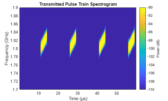
The ground surveillance radar is unaware of the direction of the target, therefore, it needs to scan the entire space to look for the aircraft. In general, the radar will transmit a series of pulses at each direction before moving to the next direction. Therefore, without losing generality, this example assumes that the radar is transmitting toward zero degrees azimuth and elevation. The following figure shows the time frequency representation of the arrival of a four-pulse train at the aircraft. Note that although the pulse train arrives at a specific delay, the time delay of the arrival of the first pulse is irrelevant for the RWR because it has no knowledge transmit time and has to constantly monitor its environment.
% Transmit a train of pulses
numPulses = 4;
txPulseTrain = helperRWR('simulateTransmission',numPulses, wavGen, rwrPos, ...
    radarPos, rwrVel, radarVel, rwrPose, radarPose, tx, radiator, envIn,fs,fc,PRF);

% Observe the signal arriving at the RWR
pspectrum(txPulseTrain,fs,'spectrogram','FrequencyLimits',[1.7e9 1.9e9], 'Leakage',0.65)
title('Transmitted Pulse Train Spectrogram')
caxis([-110 -90])
The RWR is equipped with a 10-by-10 uniform rectangular array with a spacing of /2 between its elements. It operates in the entire L-band, with a center frequency of 2 GHz. The RWR listens to the environment, and continuously feeds the collected data into the processing chain.
% Configure the receive antenna
dip = phased.IsotropicAntennaElement('BackBaffled',true);
antennaRx = phased.URA('ElementSpacing',repmat((c/2e9)/2,1,2),'Size', [10,10],'Element',dip);

% Model the radar receiver chain
collector = phased.Collector('Sensor', antennaRx,'OperatingFrequency',fc);
rx = phased.ReceiverPreamp('Gain',0,'NoiseMethod','Noise power', 'NoisePower',2.5e-6,'SeedSource','Property', 'Seed',2018);

% Collect the waves at the receiver
[~, tgtAng] = rangeangle(radarPos,rwrPos);
yr = collector(txPulseTrain,tgtAng);
yr = rx(yr);
RWR Envelope Detector
The envelope detector in the RWR is responsible for detecting the presence of any signal. As the RWR is continuously receiving data, the receiver chain buffers and truncates the received data into 50 segments.
% Truncate the received data
truncTime = 50e-6;
truncInd = round(truncTime*fs);
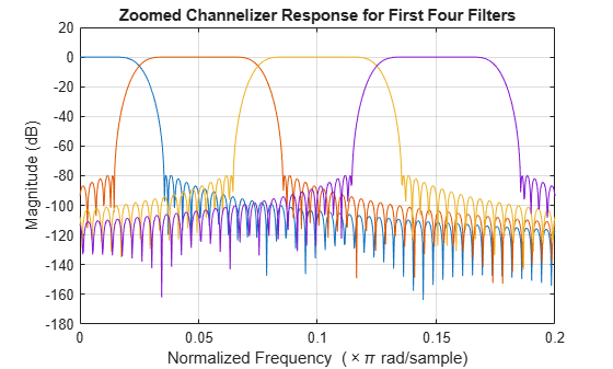
yr = yr(1:truncInd,:);Since the RWR has no knowledge about the exact center frequency used in the transmit waveform, it first uses a bank of filters, each tuned to a slightly different RF center frequency, to divide the received data into subbands. Then the envelope detector is applied in each band to check whether a signal is present. In this example, the signal is divided into subbands of 100 MHz bandwidth. An added benefit for such an operation is that instead of sampling the entire bandwidth covered by the RWR, the signal in each subband can be downsampled to a sampling frequency of 100 MHz.
% Define the bandwidth of each frequency subband
stepFreq = 100e6;

% Calculate number of subbands and configure dsp.Channelizer
numChan = fs/stepFreq;
channelizer = dsp.Channelizer('NumFrequencyBands', numChan, 'StopbandAttenuation', 80);
This plot shows the first four band created by the filter bank.
% Visualize the first four filters created in the filter bank of the
% channelizer
freqz(channelizer, 1:4)
title('Zoomed Channelizer Response for First Four Filters')
xlim([0 0.2])
% Pass the received data through the channelizer
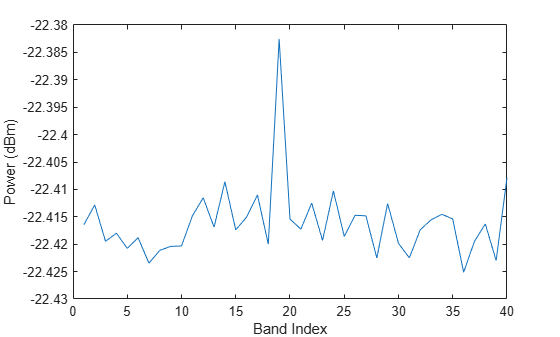
subData = channelizer(yr);The received data, subData, has three dimensions. The first dimension represents the fast-time, the second dimension represents the subbands, and the third dimension corresponds to the receiving elements of the receiving array. For the RWR's 10-by-10 antenna configuration used in this example, you have 100 receiving elements. Because the transmit power is low and the receiver noise is high, the radar signal is indistinguishable from the noise. Therefore the received powers are summed across these elements to enhance the signal-to-nose ratio (SNR) and get a better estimate of the power in each subband. The band that has the maximum power is the one used by the radar.
% Rearrange the subData to combine the antenna array channels only
incohsubData = pulsint(permute(subData,[1,3,2]),'noncoherent');
incohsubData = squeeze(incohsubData);

% Plot power distribution
subbandPow = pow2db(rms(incohsubData,1).^2)+30;
plot(subbandPow);
xlabel('Band Index');
ylabel('Power (dBm)');
% Find the subband with maximum power
[~,detInd] = max(subbandPow);
RWR Signal Processor
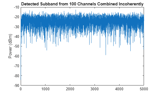
Although the power in the selected band is higher compared to the neighboring band, the SNR within the band is still low, as shown in the following figure.
subData = (subData(:,detInd,:));
subData = squeeze(subData);  % adjust the data to 2-D matrix

% Visualize the detected sub-band data
plot(mag2db(abs(sum(subData,2)))+30)
ylabel('Power (dBm)')
title('Detected Subband from 100 Channels Combined Incoherently')
% Find the original starting frequency of the sub-band having the detected
% signal
detfBand = fs*(detInd-1)/(fs/stepFreq);

% Update the sampling frequency to the decimated frequency
fs = stepFreq;
The subData is now a two-dimensional matrix. The first dimension represents fast-time samples and the second dimension is the data across 100 receiving antenna channels. The detected subband starting frequency is calculated to find the carrier frequency of the detected signal.
The next step for the RWR is to find the direction from which the radio waves are arriving. This angle of arrival information will be used to steer the receive antenna beam in the direction of the emitter and locate the emitter on the ground using single baseline approach. The RWR estimates the direction of arrival using a two-dimensional MUSIC estimator. Beam steering is done using phase-shift beamformer to achieve maximum SNR of the signal, and thus help in waveform parameter extraction.
Assume that the ground plane is flat and parallel to the xy-plane of the coordinate system. Then, the RWR can use the altitude information from its altimeter readings of the aircraft along with the direction of arrival to triangulate the location of the emitter.
% Configure the MUSIC Estimator to find the direction of arrival of the
% signal
doaEst = phased.MUSICEstimator2D('OperatingFrequency',fc,'PropagationSpeed',c,...
    'SensorArray',antennaRx,'DOAOutputPort',true,'AzimuthScanAngles',-50:.5:50,...
    'ElevationScanAngles',-50:.5:50, 'NumSignalsSource', 'Property','NumSignals', 1);

[mSpec,doa] = doaEst(subData);
plotSpectrum(doaEst,'Title','2-D MUSIC Spatial Spectrum Top View');
view(0,90); axis([-30 0 -30 0]);
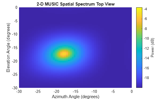
The figure clearly shows the location of the emitter.
% Configure the beamformer object to steer the beam before combining the
% channels
beamformer = phased.PhaseShiftBeamformer('SensorArray',antennaRx,...
    'OperatingFrequency',fc,'DirectionSource','Input port');

% Apply the beamforming, and visualize the beam steered radiation
% pattern
mBeamf = beamformer(subData, doa);

% Find the location of the emitter
altimeterElev = rwrPos(3);
d = abs(altimeterElev/sind(doa(2)));
After applying the beam steering, the antenna has the maximum gain in the azimuth and elevation angle of the arrival of the signal. This further improves the SNR of the intercepted signal. Next, the signal parameters are extracted in the signal processor using one of the time-frequency analysis techniques known as pseudo Wigner-Ville transform coupled with Hough transform as described in [2].
First, derive the time frequency representation of the intercepted signal using the Wigner-Ville transform.
% Compute the pseudo Wigner-Ville transform
[tpwv,t,f] = helperRWR('pWignerVille',mBeamf,fs);

% Plot the pseudo Wigner-Ville transform
imagesc(f*1e-6,t*1e6,pow2db(abs(tpwv./max(tpwv(:)))));
xlabel('Frequency (MHz)'); ylabel('Time(\mus)');
caxis([-50 0]); clb = colorbar; clb.Label.String = 'Normalized Power (dB)';
title ('Pseudo Wigner-Ville Transform')
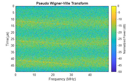
Using human eyes, even though the resulting time frequency representation is noisy, it is not too hard to separate the signal from the background. Each pulse appears as a line in the time frequency plane. Thus, using beginning and end of the time-frequency lines, you can derive the pulse width and the bandwidth of the pulse. Similarly, the time between lines from different pulses gives you the pulse repetition interval.
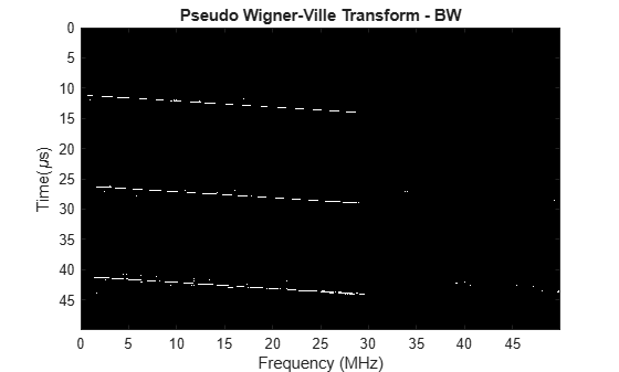
To do this automatically without relying on human eyes, use Hough transform to identify those lines from the image. The Hough transform can perform well in the presence of noise, and the transform is an enhancement to the time-frequency signal analysis method.
To use the Hough transform, it is necessary to convert the time frequency image into a binary image. The following performs some data smoothing on the image and then uses the imbinarize function to do the conversion. The conversion threshold can be modified based on the signal-noise characteristics of the receiver and the operating environment.
% Normalize the pseudo Wigner-Ville image
twvNorm = abs(tpwv)./max(abs(tpwv(:)));

% Implement a median filter to clear the noise
filImag = medfilt2(twvNorm,[7 7]);

% Use threshold to convert filtered image into binary image
BW = imbinarize(filImag./max(filImag(:)), 0.15);
imagesc(f*1e-6,t*1e6,BW); colormap('gray');
xlabel('Frequency (MHz)'); ylabel('Time(\mus)');
title ('Pseudo Wigner-Ville Transform - BW')
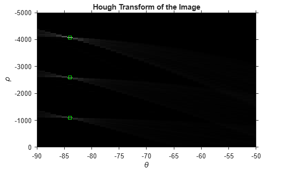
Using the Hough transform, the binary pseudo Wigner-Ville image is first transformed to peaks. This way, instead of detecting the line in an image, you just need to detect a peak in an image.
% Compute the Hough transform of the image and plot
[H,T,R] = hough(BW);
imshow(H,[],'XData',T,'YData',R,'InitialMagnification','fit');
xlabel('\theta'), ylabel('\rho');
axis on, axis normal, hold on;
title('Hough Transform of the Image')
The peak positions are extracted using the houghpeaks function.
% Compute peaks in the transform, up to 5 peaks
P  = houghpeaks(H,5);
x = T(P(:,2)); y = R(P(:,1));
plot(x,y,'s','color','g'); xlim([-90 -50]); ylim([-5000 0])
Using these positions, the houghlines function can reconstruct the lines in the original binary image. Then as discussed earlier, the beginning and the end of these lines help you estimate the waveform parameters.
lines = houghlines(BW,T,R,P,'FillGap',3e-6*fs,'MinLength',1e-6*fs);
coord = [lines(:).point1; lines(:).point2];

% Plot the detected lines superimposed on the binary image
clf;
imagesc(f*1e-6, t*1e6, BW); colormap(gray); hold on
xlabel('Frequency (MHz)')
ylabel('Time(\mus)')
title('Hough Transform — Detected Lines')
for ii = 1:2:2*size(lines,2)
    plot(f(coord(:,ii))*1e-6, t(coord(:,ii+1))*1e6,'LineWidth',2,'Color','green');
end
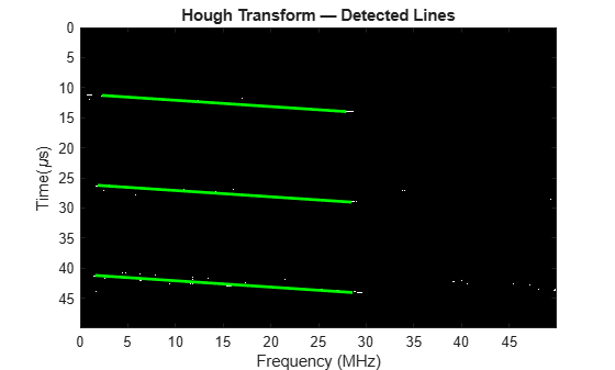
% Calculate the parameters using the line co-ordinates
pulDur = t(coord(2,2)) - t(coord(1,2));         % Pulse duration
bWidth = f(coord(2,1)) - f(coord(1,1));         % Pulse Bandwidth
pulRI = abs(t(coord(1,4)) - t(coord(1,2)));     % Pulse repetition interval
detFc = detfBand + f(coord(2,1));               % Center frequency
The extracted waveform characteristics are listed next. They match the truth very well. These estimates can then be used to catalog the radar and prepare for counter measures if necessary.
helperRWR('displayParameters',pulRI, pulDur, bWidth,detFc, doa,d);Pulse repetition interval = 14.97 microseconds Pulse duration = 2.84 microseconds Pulse bandwidth = 27 MHz Center frequency = 1.8286 GHz Azimuth angle of emitter = -18.5 degrees Elevation angle of emitter = -17.5 degrees Distance of the emitter = 3325.5095 m
Summary
This example shows how an RWR can estimate the parameters of the intercepted radar pulse using signal processing and image processing techniques.
References
[1] Electronic Warfare and Radar Systems Engineering Handbook 2013, Naval Air Warfare Center Weapons Division, Point Mugu, California.
[2] Stevens, Daniel L., and Stephanie A. Schuckers. “Detection and Parameter Extraction of Low Probability of Intercept Radar Signals Using the Hough Transform.” Global Journal of Researches in Engineering, Jan. 2016, pp. 9–25. DOI.org (Crossref), https://doi.org/10.34257/GJREJVOL15IS6PG9.