Model-Based Reinforcement Learning Using Custom Training Loop
This example shows how to define a custom training loop for a model-based reinforcement learning (MBRL) algorithm. You can use this workflow to train an MBRL policy with your custom training algorithm using policy and value function approximators from Reinforcement Learning Toolbox™ software.
For an example on how to use the built in model-based policy optimization (MBPO) agent, see Train MBPO Agent to Balance Continuous Cart-Pole System. For an overview of built-in MBPO agents, see Model-Based Policy Optimization (MBPO) Agent.
In this example, you use transition models to generate more experiences while training a custom DQN [2] agent in a cart-pole environment. The algorithm used in this example is based on an MBPO algorithm [1]. The original MBPO algorithm trains an ensemble of stochastic models and a soft actor-critic (SAC) agent in tasks with continuous actions. In contrast, this example trains three deterministic models and a DQN agent in a task with discrete actions. The following figure summarizes the algorithm used in this example.
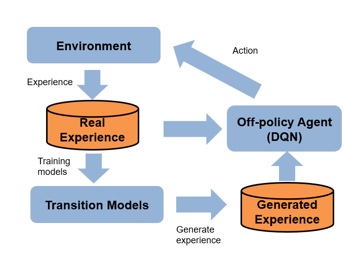
The agent generates real experiences by interacting with the environment. These experiences are used to train a set of transition models, which are used to generate additional experiences. The training algorithm then uses both the real and generated experiences to update the agent policy.
Create Environment
For this example, a reinforcement learning policy is trained in a discrete cart-pole environment. The objective in this environment is to balance the pole by applying forces (actions) on the cart. Create the environment using the rlPredefinedEnv function. Fix the random generator seed for reproducibility. For more information on this environment, see Use Predefined Control System Environments.
clear
clc
rngSeed = 1;
rng(rngSeed);
env = rlPredefinedEnv("CartPole-Discrete");
Extract the observation and action specifications from the environment.
obsInfo = getObservationInfo(env);
actInfo = getActionInfo(env);
Obtain the number of observations (numObservations) and actions (numActions).
numObservations = obsInfo.Dimension(1);
% Number of discrete actions, -10 or 10
numActions = numel(actInfo.Elements);
numContinuousActions = 1; % force
Critic Construction
DQN agents use a parameterized Q-value function approximator to estimate the value of the policy. Because DQN agents have a discrete action space, you have the option to create a vector (that is, multi-output) Q-value function critic, which is generally more efficient than a comparable single-output critic.
A vector Q-value function takes only the observation as input and returns as output a single vector with as many elements as the number of possible actions. The value of each output element represents the expected discounted cumulative long-term reward when an agent starts from the state corresponding to the given observation and executes the action corresponding to the element number (and follows the given policy afterwards).
To model the parameterized Q-value function within the critic, use a neural network. For more information about the layers, see fullyConnectedLayer, and reluLayer.
qNetwork = [
    featureInputLayer(obsInfo.Dimension(1))
    fullyConnectedLayer(24)
    reluLayer
    fullyConnectedLayer(24)
    reluLayer
    fullyConnectedLayer(length(actInfo.Elements))
    ];
Convert to dlnetwork object.
qNetwork = dlnetwork(qNetwork);
Display the number of learnable parameters.
summary(qNetwork)
   Initialized: true

   Number of learnables: 770

   Inputs:
      1   'input'   4 features
Create the critic using the specified neural network and options. For more information, rlVectorQValueFunction.
critic = rlVectorQValueFunction(qNetwork,obsInfo,actInfo);
Create optimizer objects for updating the critic. For more information, see rlOptimizerOptions.
optimizerOpt = rlOptimizerOptions( ...
    LearnRate=1e-3, ...
    GradientThreshold=1);
criticOptimizer = rlOptimizer(optimizerOpt);
Create a max Q value policy.
policy = rlMaxQPolicy(critic);
Create Transition Models
Model-based reinforcement learning uses transition models of the environment. The model usually consists of a transition function, a reward function, and a terminal state function.
The transition function predicts the next observation given the current observation and the action.
The reward function predicts the reward given the current observation, the action, and the next observation.
The terminal state function predicts the terminal state given the observation.
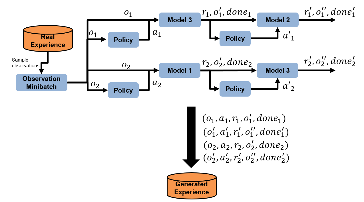
As shown in the following figure, this example uses three transition functions as an ensemble of transition models to generate samples without interacting with the environment. The true reward function and the true terminal state function are given in this example.
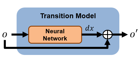
Define three neural networks for transition models. The neural network predicts the difference between the next observation and the current observation.
numModels = 3;
transitionNetwork1 = ...
   createTransitionNetwork(numObservations, numContinuousActions);

transitionNetwork2 = ...
   createTransitionNetwork(numObservations, numContinuousActions);

transitionNetwork3 = ...
   createTransitionNetwork(numObservations, numContinuousActions);

transitionNetworkVector =   [transitionNetwork1, ...
                             transitionNetwork2, ...
                             transitionNetwork3];
Create Experience Buffers
Create an experience buffer for storing agent experiences (observation, action, next observation, reward, and isDone).
myBuffer.bufferSize = 1e5;
myBuffer.bufferIndex = 0;
myBuffer.currentBufferLength = 0;
myBuffer.observation = zeros(numObservations,myBuffer.bufferSize);
myBuffer.nextObservation = ...
                       zeros(numObservations,myBuffer.bufferSize);
myBuffer.action = ...
    zeros(numContinuousActions,1,myBuffer.bufferSize);
myBuffer.reward = zeros(1,myBuffer.bufferSize);
myBuffer.isDone = zeros(1,myBuffer.bufferSize);
Create a model experience buffer for storing the experiences generated by the models.
myModelBuffer.bufferSize = 1e5;
myModelBuffer.bufferIndex = 0;
myModelBuffer.currentBufferLength = 0;
myModelBuffer.observation =...
    zeros(numObservations,myModelBuffer.bufferSize);
myModelBuffer.nextObservation =...
    zeros(numObservations,myModelBuffer.bufferSize);
myModelBuffer.action = ...
    zeros(numContinuousActions,myModelBuffer.bufferSize);
myModelBuffer.reward = zeros(1,myModelBuffer.bufferSize);
myModelBuffer.isDone = zeros(1,myModelBuffer.bufferSize);
Configure Training
Configure the training to use the following options.
Maximum number of training episodes — 250
Maximum steps per training episode — 500
Discount factor — 0.99
Training termination condition — Average reward across 10 episodes reaches the value of 480
numEpisodes = 250;
maxStepsPerEpisode = 500;
discountFactor = 0.99;
aveWindowSize = 10;
trainingTerminationValue = 480;
Configure the model options.
Train transition models only after 2000 samples are collected.
Train the models using all experiences in the real experience buffer in each episode. Use a mini-batch size of 256.
The models generate trajectories with a length of 2 at the beginning of each episode.
The number of generated trajectories is
numGenerateSampleIterationxnumModelsxminiBatchSize= 20 x 3 x 256 = 15360.Use the same epsilon-greedy parameters as the DQN agent, except for the minimum epsilon value.
Use a minimum epsilon value of 0.1, which is higher than the value used for interacting with the environment. Doing so allows the model to generate more diverse data.
warmStartSamples = 2000;
numEpochs = 1;
miniBatchSize = 256;
horizonLength = 2;
epsilonMinModel = 0.1;
numGenerateSampleIteration = 20;
sampleGenerationOptions.horizonLength = horizonLength;
sampleGenerationOptions.numGenerateSampleIteration = ...
                             numGenerateSampleIteration;
sampleGenerationOptions.miniBatchSize = miniBatchSize;
sampleGenerationOptions.numObservations = numObservations;
sampleGenerationOptions.epsilonMinModel = epsilonMinModel;

% optimizer options
velocity1 = [];
velocity2 = [];
velocity3 = [];
decay = 0.01;
momentum = 0.9;
learnRate = 0.0005;
Configure the DQN training options.
Use the epsilon greedy algorithm with an initial epsilon value is 1, a minimum value of 0.01, and a decay rate of 0.005.
Update the target network every 4 steps.
Set the ratio of the real experiences to generated experiences to 0.2:0.8 by setting
RealRatioto 0.2. SettingRealRatioto 1.0 is the same as the model-free DQN.Take 5 gradient steps at each environment step.
epsilon = 1;
epsilonMin = 0.01;
epsilonDecay = 0.005;
targetUpdateFrequency = 4;
realRatio = 0.2; % Set to 1 to run a standard DQN
numGradientSteps = 5;
Create a vector for storing the cumulative reward for each training episode.
episodeCumulativeRewardVector = [];
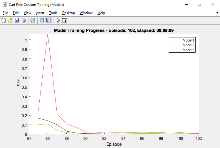
Create a figure for model training visualization using the hBuildFigureModel helper function.
[trainingPlotModel, ...
    lineLossTrain1, ...
    lineLossTrain2, ...
    lineLossTrain3, ...
    axModel] = hBuildFigureModel();
Create a figure for model validation visualization using the hBuildFigureModelTest helper function.
[testPlotModel, lineLossTest1, axModelTest] ...
                                 = hBuildFigureModelTest();
Create a figure for DQN agent training visualization using the hBuildFigure helper function.
[trainingPlot,lineReward,lineAveReward, ax] = hBuildFigure;
Train Agent
Train the agent using a custom training loop. The training loop uses the following algorithm. For each episode:
Train the transition models.
Generate experiences using the transition models and store the samples in the model experience buffer.
Generate a real experience. To do so, generate an action using the policy, apply the action to the environment, and obtain the resulting observation, reward, and is-done values.
Create a mini-batch by sampling experiences from both the experience buffer and the model experience buffer.
Compute the target Q value.
Compute the gradient of the loss function with respect to the critic parameters.
Update the critic using the computed gradients.
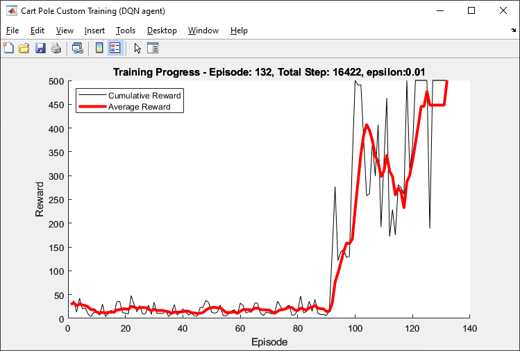
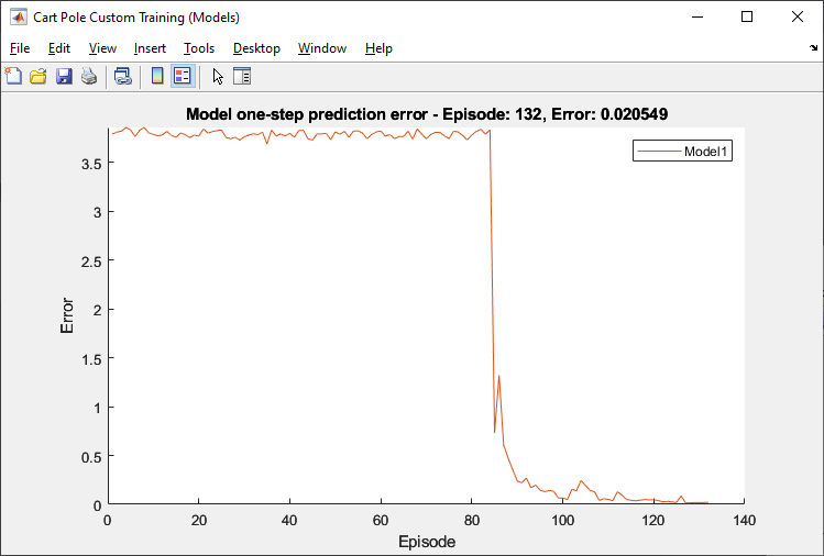
Update the training visualization.
Terminate training if the critic is sufficiently trained.
Training the policy is a computationally intensive process. To save time while running this example, load a pretrained agent by setting doTraining to false. To train the policy yourself, set doTraining to true.
doTraning = false;
if doTraning
    targetCritic = critic;
    modelTrainedAtleastOnce = false;
    totalStepCt = 0;
    start = tic;

    set(trainingPlotModel,Visible = "on");
    set(testPlotModel,Visible = "on");
    set(trainingPlot,Visible = "on");

    for episodeCt = 1:numEpisodes
        if myBuffer.currentBufferLength > miniBatchSize && ...
                totalStepCt > warmStartSamples
            if realRatio < 1.0
                %----------------------------------------------
                % 1. Train transition models.
                %----------------------------------------------
                % Training three transition models
                [transitionNetworkVector(1),loss1,velocity1] = ...
                        trainTransitionModel( ...
                        transitionNetworkVector(1), ...
                        myBuffer,velocity1,miniBatchSize, ...
                        numEpochs,momentum,learnRate);
                [transitionNetworkVector(2),loss2,velocity2] = ...
                        trainTransitionModel( ...
                        transitionNetworkVector(2), ...
                        myBuffer,velocity2,miniBatchSize, ...
                        numEpochs,momentum,learnRate);
                [transitionNetworkVector(3),loss3,velocity3] = ...
                        trainTransitionModel( ...
                        transitionNetworkVector(3), ...
                        myBuffer,velocity3,miniBatchSize, ...
                        numEpochs,momentum,learnRate);
                modelTrainedAtleastOnce = true;

                % Display the training progress
                d = duration(0,0,toc(start),"Format",'hh:mm:ss');
                addpoints(lineLossTrain1,episodeCt,loss1)
                addpoints(lineLossTrain2,episodeCt,loss2)
                addpoints(lineLossTrain3,episodeCt,loss3)
                legend(axModel,"Model1","Model2","Model3");
                title(axModel, ...
                    "Model Training Progress - Episode: "...
                    + episodeCt + ", Elapsed: " + string(d))
                drawnow

                %----------------------------------------------
                % 2. Generate experience using models.
                %----------------------------------------------
                % Create numGenerateSampleIteration x
                % horizonLength xnumModels x miniBatchSize
                % ex) 20 x 2 x 3 x 256 = 30720 samples
                myModelBuffer = generateSamples(myBuffer, ...
                    myModelBuffer, ...
                    transitionNetworkVector,policy,actInfo, ...
                    epsilon,sampleGenerationOptions);
            end
        end

        %----------------------------------------------
        % Interact with environment and train agent.
        %----------------------------------------------
        % Reset the environment at the start of the episode
        observation = reset(env);
        episodeReward = zeros(maxStepsPerEpisode,1);
        errorPreddiction = zeros(maxStepsPerEpisode,1);

        for stepCt = 1:maxStepsPerEpisode
            %----------------------------------------------
            % 3. Generate an experience.
            %----------------------------------------------
            totalStepCt = totalStepCt + 1;

            % Compute an action using the policy based on
            % the current observation.
            if rand() < epsilon
                action = actInfo.usample;
            else
                action = getAction(policy,{observation});
            end
            action = action{1};
            % Udpate epsilon
            if totalStepCt > warmStartSamples
                epsilon = max(epsilon*(1-epsilonDecay), ...
                              epsilonMin);
            end

            % Apply the action to the environment and obtain the
            % resulting observation and reward.
            [nextObservation,reward,isDone] = step(env,action);

            % Check prediction
            dx = predict(transitionNetworkVector(1), ...
                dlarray(observation,"CB"),dlarray(action,"CB"));
            predictedNextObservation = observation + dx;
            errorPreddiction(stepCt) = ...
                sqrt(sum((nextObservation - ...
                                predictedNextObservation).^2));

            % Store the action, observation, reward and is-done
            % experience
            myBuffer = storeExperience(myBuffer, ...
                                observation, ...
                                action, ...
                                nextObservation,reward,isDone);

            episodeReward(stepCt) = reward;
            observation = nextObservation;

            % Train DQN agent
            for gradientCt = 1:numGradientSteps
                if myBuffer.currentBufferLength >= miniBatchSize ...
                        && totalStepCt>warmStartSamples
                    %----------------------------------------------
                    % 4. Sample mini-batch from experience buffers.
                    %----------------------------------------------
                    [sampledObservation, ...
                        sampledAction, ...
                        sampledNextObservation, ...
                        sampledReward, ...
                        sampledIsdone] ...
                              = sampleMinibatch( ...
                                    modelTrainedAtleastOnce, ...
                                    realRatio, ...
                                    miniBatchSize, ...
                                    myBuffer,myModelBuffer);

                    %----------------------------------------------
                    % 5. Compute target Q value.
                    %----------------------------------------------
                    % Compute target Q value
                    [targetQValues, MaxActionIndices] = ...
                            getMaxQValue(targetCritic, ...
                            {reshape(sampledNextObservation, ...
                            [numObservations,1,miniBatchSize])});

                    % Compute target for nonterminal states
                    targetQValues(~logical(sampledIsdone)) = ...
                        sampledReward(~logical(sampledIsdone)) + ...
                        discountFactor.* ...
                        targetQValues(~logical(sampledIsdone));
                    % Compute target for terminal states
                    targetQValues(logical(sampledIsdone)) = ...
                        sampledReward(logical(sampledIsdone));

                    lossData.batchSize = miniBatchSize;
                    lossData.actInfo = actInfo;
                    lossData.actionBatch = sampledAction;
                    lossData.targetQValues = targetQValues;

                    %----------------------------------------------
                    % 6. Compute gradients.
                    %----------------------------------------------
                    criticGradient = ...
                        gradient(critic, ...
                             @criticLossFunction, ...
                            {reshape(sampledObservation, ...
                            [numObservations,1,miniBatchSize])}, ...
                            lossData);

                    %----------------------------------------------
                    % 7. Update the critic network using gradients.
                    %----------------------------------------------
                    [critic, criticOptimizer] = update( ...
                        criticOptimizer, critic, ...
                        criticGradient);

                    % Update the policy parameters using the critic
                    % parameters.
                    policy = setLearnableParameters( ...
                                    policy, ...
                                    getLearnableParameters(critic));
                end
            end
            % Update target critic periodically
            if mod(totalStepCt, targetUpdateFrequency)==0
                targetCritic = critic;
            end

            % Stop if a terminal condition is reached.
            if isDone
                break;
            end
        end % End of episode

        %---------------------------------------------------------
        % 8. Update the training visualization.
        %---------------------------------------------------------
        episodeCumulativeReward = sum(episodeReward);
        episodeCumulativeRewardVector = cat(2, ...
            episodeCumulativeRewardVector,episodeCumulativeReward);
        movingAveReward = movmean(episodeCumulativeRewardVector, ...
            aveWindowSize,2);
        addpoints(lineReward,episodeCt,episodeCumulativeReward);
        addpoints(lineAveReward,episodeCt,movingAveReward(end));
        title(ax, "Training Progress - Episode: " + episodeCt + ...
            ", Total Step: " + string(totalStepCt) + ...
            ", epsilon:" + string(epsilon))
        drawnow;

        errorPreddiction = errorPreddiction(1:stepCt);

        % Display one step prediction error.
        addpoints(lineLossTest1,episodeCt,mean(errorPreddiction))
        legend(axModelTest,"Model1");
        title(axModelTest, ...
            "Model one-step prediction error - Episode: " + ...
            episodeCt + ", Error: " + ...
            string(mean(errorPreddiction)))
        drawnow

        % Display training progress every 10th episode
        if (mod(episodeCt,10) == 0)
            fprintf("EP:%d, Reward:%.4f, AveReward:%.4f, " + ...
                    "Steps:%d, TotalSteps:%d, epsilon:%f," + ...
                    "error model:%f\n", ...
                        episodeCt, ...
                        episodeCumulativeReward, ...
                        movingAveReward(end), ...
                        stepCt,totalStepCt, ...
                        epsilon, ...
                        mean(errorPreddiction))
        end

        %---------------------------------------------------------
        % 9. Terminate training
        %    if the network is sufficiently trained.
        %---------------------------------------------------------
        if max(movingAveReward) > trainingTerminationValue
            break
        end
    end
else
    load("cartPoleModelBasedCustomLoopPolicy.mat");
end
Simulate Agent
To simulate the trained agent, first reset the environment.
obs0 = reset(env);
obs = obs0;
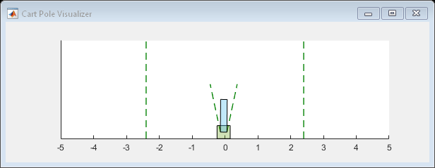
Enable the environment visualization, which is updated each time the environment step function is called.
plot(env)
For each simulation step, perform the following actions.
Get the action by sampling from the policy using the
getActionfunction.Step the environment using the obtained action value.
Terminate if a terminal condition is reached.
actionVector = zeros(1,maxStepsPerEpisode);
obsVector = zeros(numObservations,maxStepsPerEpisode+1);
obsVector(:,1) = obs0;
for stepCt = 1:maxStepsPerEpisode

    % Select action according to trained policy.
    action = getAction(policy,{obs});
    action= action{1};

    % Step the environment.
    [nextObs,reward,isDone] = step(env,action);

    obsVector(:,stepCt+1) = nextObs;
    actionVector(1,stepCt) = action;

    % Check for terminal condition.
    if isDone
        break
    end

    obs = nextObs;
end
lastStepCt = stepCt;
Test Model
Test one of the models by predicting a next observation given a current observation and an action.
modelID = 3;
predictedObsVector = zeros(numObservations,lastStepCt);
obs = dlarray(obsVector(:,1),"CB");
predictedObsVector(:,1) = obs;
for stepCt = 1:lastStepCt
    obs = dlarray(obsVector(:,stepCt),"CB");
    action = dlarray(actionVector(1,stepCt),"CB");

    dx = predict(transitionNetworkVector(modelID),obs, action);
    predictedObs = obs + dx;
    predictedObsVector(:,stepCt+1) = predictedObs;
end
predictedObsVector = predictedObsVector(:, 1:lastStepCt);
figure(5)
layOut = tiledlayout(4,1, "TileSpacing", "compact");
for i = 1:4
    nexttile;
    errorPrediction = abs(predictedObsVector(i,1:lastStepCt) - ...
                                        obsVector(i,1:lastStepCt));
    line1 = plot(errorPrediction,"DisplayName", "Absolute Error");
    title("observation "+num2str(i));
end
title(layOut,"Prediction Absolute Error")
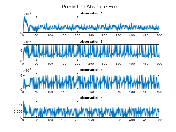
The small absolute prediction error shows that the model is successfully trained to predict the next observation.
References
[1] Minh, Volodymyr, Koray Kavukcuoglu, David Silver, Alex Graves, Ioannis Antonoglou, Daan Wierstra, and Martin Riedmiller. “Playing Atari with Deep Reinforcement Learning.” Preprint, submitted December 19, 2013. https://arxiv.org/abs/1312.5602.
[2] Janner, Michael, Justin Fu, Marvin Zhang, and Sergey Levine. "When to trust your model: Model-based policy optimization." Preprint, submitted November 5, 2019. https://arxiv.org/abs/1906.08253.