Train DQN Agent for Lane Keeping Assist

This example shows how to train a deep Q-learning network (DQN) agent for lane keeping assist (LKA) in Simulink®. For more information on DQN agents, see Deep Q-Network (DQN) Agents.

Simulink Model for Ego Car

The reinforcement learning environment for this example is a simple bicycle model for the ego vehicle dynamics. The training goal is to keep the ego vehicle traveling along the centerline of the lanes by adjusting the front steering angle. This example uses the same vehicle model as in Lane Keeping Assist System Using Model Predictive Control (Model Predictive Control Toolbox). The ego car dynamics is specified by the following parameters.

m = 1575;   % total vehicle mass (kg)
Iz = 2875;  % yaw moment of inertia (mNs^2)
lf = 1.2;   % longitudinal distance from center of gravity to front tires (m)
lr = 1.6;   % longitudinal distance from center of gravity to rear tires (m)
Cf = 19000; % cornering stiffness of front tires (N/rad)
Cr = 33000; % cornering stiffness of rear tires (N/rad)
Vx = 15;    % longitudinal velocity (m/s)

Define the sample time Ts and simulation duration Tf in seconds.

Ts = 0.1;
T = 15;

The output of the LKA system is the front steering angle of the ego car. To simulate the physical limitations of the ego car, constrain the steering angle to the range [-0.5,0.5] rad.

u_min = -0.5;
u_max = 0.5;

The curvature of the road is defined by a constant 0.001 ($$m^{-1}$$). The initial value for the lateral deviation is 0.2 m and the initial value for the relative yaw angle is –0.1 rad.

rho = 0.001;
e1_initial = 0.2;
e2_initial = -0.1;

Open the model.

mdl = "rlLKAMdl";
open_system(mdl);
agentblk = mdl + "/RL Agent";

For this model:

• The steering-angle action signal from the agent to the environment is from –15 degrees to 15 degrees.

• The observations from the environment are the lateral deviation ${\mathit{e}}_1$, the relative yaw angle ${\mathit{e}}_2$, their derivatives $${\underset{}{\overset{\dot{}}{e}}}_1$$ and $${\underset{}{\overset{\dot{}}{e}}}_2$$, and their integrals $\int {\mathit{e}}_1$ and $\int {\mathit{e}}_2$.

• The simulation is terminated when the lateral deviation $$|e_1|>1.$$

• The reward ${\mathit{r}}_{\mathit{t}}$, provided at every time step $\mathit{t}$, is

$$r_t=-(10e_1^2+5e_2^2+2u^2+5{\underset{}{\overset{\dot{}}{e}}}_1^2+5{\underset{}{\overset{\dot{}}{e}}}_2^2)$$

where $\mathit{u}$ is the control input from the previous time step $\mathit{t}-1$.

Create Environment Interface

Create a reinforcement learning environment interface for the ego vehicle. To do so, first create the observation and action specifications.

observationInfo = rlNumericSpec([6 1], ...
    LowerLimit=-inf*ones(6,1), ...
    UpperLimit=inf*ones(6,1));
observationInfo.Name = "observations";
observationInfo.Description = "Lateral deviation and relative yaw angle";
actionInfo = rlFiniteSetSpec((-15:15)*pi/180);
actionInfo.Name = "steering";

Then, create the environment interface.

env = rlSimulinkEnv(mdl,agentblk,observationInfo,actionInfo);

The interface has a discrete action space where the agent can apply one of 31 possible steering angles from –15 degrees to 15 degrees. The observation is the six-dimensional vector containing lateral deviation, relative yaw angle, as well as their derivatives and integrals with respect to time.

To define the initial condition for lateral deviation and relative yaw angle, specify an environment reset function using an anonymous function handle. This reset function randomizes the initial values for the lateral deviation and relative yaw angle.

env.ResetFcn = @(in)localResetFcn(in);

Fix the random generator seed for reproducibility.

rng(0)

Create DQN agent

DQN agents use a parametrized Q-value function approximator to estimate the value of the policy.

Since DQN agents have a discrete action space, you have the option to create a vector (that is multi-output) Q-value function critic, which is generally more efficient than a comparable single-output critic

A vector Q-value function takes only the observation as input and returns as output a single vector with as many elements as the number of possible actions. The value of each output element represents the expected discounted cumulative long-term reward when an agent starts from the state corresponding to the given observation and executes the action corresponding to the element number (and follows a given policy afterwards)

To model the parametrized Q-value function within the critic, use a deep neural network with one input (the six-dimensional observed state) and one output vector with 31 elements (evenly spaced steering angles from -15 to 15 degrees).

% Define number of inputs, neurons, and outputs
nI = observationInfo.Dimension(1);  % number of inputs (6)
nL = 24;                            % number of neurons
nO = numel(actionInfo.Elements);    % number of outputs (31)

% Define network as array of layer objects
dnn = [
    featureInputLayer(nI)
    fullyConnectedLayer(nL)
    reluLayer
    fullyConnectedLayer(nL)
    reluLayer
    fullyConnectedLayer(nO)
    ];

% Convert to dlnetwork object
dnn = dlnetwork(dnn);

Display the number of parameters and view the network configuration.

summary(dnn)

   Initialized: true

   Number of learnables: 1.5k

   Inputs:
      1   'input'   6 features

plot(dnn)

Create the critic using dnn and the observation and action specifications. For more information, see rlQValueFunction.

critic = rlVectorQValueFunction(dnn,observationInfo,actionInfo);

Specify training options for the critic using rlOptimizerOptions.

criticOptions = rlOptimizerOptions( ...
    LearnRate=1e-4, ...
    GradientThreshold=1, ...
    L2RegularizationFactor=1e-4);

Specify the DQN agent options using rlDQNAgentOptions, include the training options for the critic.

agentOptions = rlDQNAgentOptions(...
    SampleTime=Ts,...
    UseDoubleDQN=true,...
    CriticOptimizerOptions=criticOptions,...
    ExperienceBufferLength=1e6,...
    MiniBatchSize=64);

Then, create the DQN agent using the specified critic representation and agent options. For more information, see rlDQNAgent.

agent = rlDQNAgent(critic,agentOptions);

Train Agent

To train the agent, first specify the training options. For this example, use the following options:

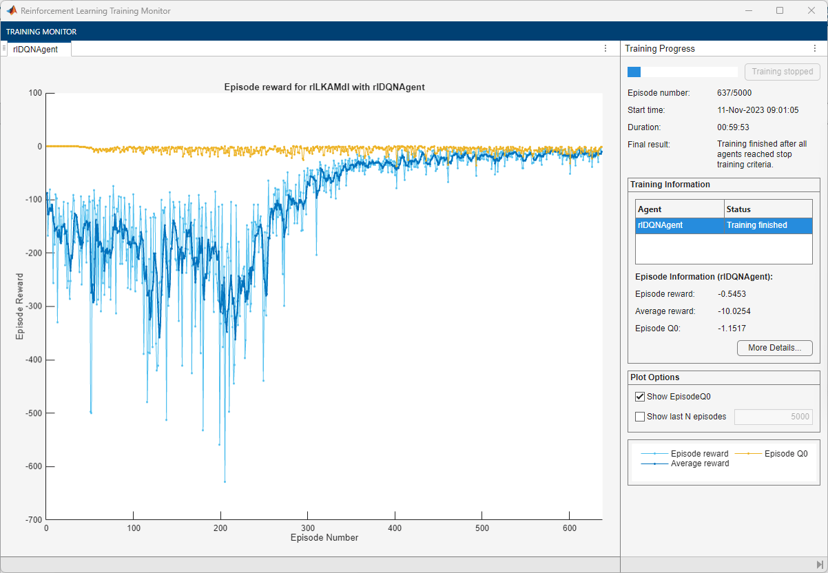
• Run each training episode for at most 5000 episodes, with each episode lasting at most ceil(T/Ts) time steps.

• Display the training progress in the Episode Manager dialog box (set the Plots option to training-progress) and disable the command line display (set the Verbose option to false).

• Stop training when the episode reward reaches –1.

• Save a copy of the agent for each episode where the cumulative reward is greater than –2.5.

For more information, see rlTrainingOptions.

maxepisodes = 5000;
maxsteps = ceil(T/Ts);
trainingOpts = rlTrainingOptions(...
    MaxEpisodes=maxepisodes,...
    MaxStepsPerEpisode=maxsteps,...
    Verbose=false,...
    Plots="training-progress",...
    StopTrainingCriteria="EpisodeReward",...
    StopTrainingValue=-1,...
    SaveAgentCriteria="EpisodeReward",...
    SaveAgentValue=-2.5);

Train the agent using the train function. Training is a computationally intensive process that takes several hours to complete. To save time while running this example, load a pretrained agent by setting doTraining to false. To train the agent yourself, set doTraining to true.

doTraining = false;

if doTraining    
    % Train the agent.
    trainingStats = train(agent,env,trainingOpts);
else
    % Load the pretrained agent for the example.
    load("SimulinkLKADQNMulti.mat","agent")       
end

Simulate DQN Agent

To validate the performance of the trained agent, uncomment the following two lines and simulate the agent within the environment. For more information on agent simulation, see rlSimulationOptions and sim.

% simOptions = rlSimulationOptions(MaxSteps=maxsteps);
% experience = sim(env,agent,simOptions);

To demonstrate the trained agent on deterministic initial conditions, simulate the model in Simulink.

e1_initial = -0.4;
e2_initial = 0.2;
sim(mdl)

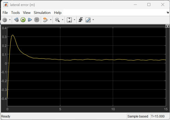
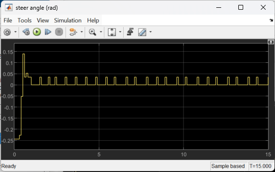
As the plots show, the lateral error (top plot) and relative yaw angle (middle plot) are both driven close to zero. The vehicle starts from off the centerline (–0.4 m) and with a nonzero yaw angle error (0.2 rad). The lane keeping assist makes the ego car travel along the centerline after about 2.5 seconds. The steering angle (bottom plot) shows that the controller reaches steady state after about 2 seconds.

Close the Simulink model.

if ~doTraining
    %bdclose(mdl)
end

Reset Function

function in = localResetFcn(in)
    % reset lateral deviation and relative yaw angle to random values
    in = setVariable(in,"e1_initial", 0.5*(-1+2*rand)); 
    in = setVariable(in,"e2_initial", 0.1*(-1+2*rand));
end