Design Broadband Matching Networks for Amplifier

Open Live Script

This example shows how to design broadband matching networks for a low noise amplifier (LNA) with ideal and real-world lumped LC elements. The real-world lumped LC elements are obtained from the Modelithics SELECT+ Library™. The LNA is designed to the target gain and noise figure specifications over a specified bandwidth. A direct-search based approach is used to arrive at the optimum element values in the input and output matching networks.

In an RF receiver front end, the LNA is commonly found immediately after the antenna or after the first bandpass filter that follows the antenna. Its position in the receiver chain ensures that it deals with weak signals that have significant noise content. As a result the LNA has to not only provide amplification to such signals but also minimize its own noise footprint on the amplified signal.

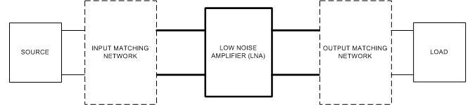
Figure 1: Impedance matching of an amplifier

Set Design Parameters

The design specifications are as follows.

Amplifier is an LNA amplifier
Center Frequency = 250 MHz
Bandwidth = 100 MHz
Transducer Gain greater than or equal to 10 dB
Noise Figure less than or equal to 2.0 dB
Operating between 50-Ohm terminations

Specify Design Parameters

You are building the matching network for an LNA with a bandpass response, so specify the bandwidth of match, center frequency, gain, and noise figure targets.

BW = 100e6;            % Bandwidth of matching network (Hz)
fc = 250e6;            % Center frequency (Hz)
Gt_target = 10;        % Transducer gain target (dB)
NFtarget = 2;          % Max noise figure target (dB)

Specify the source impedance, reference impedance, and the load impedance.

Zs = 50;               % Source impedance (Ohm)
Z0 = 50;               % Reference impedance (Ohm)
Zl = 50;               % Load impedance (Ohm)

Create Amplifier Object and Perform Analysis

Create an amplifier object from lnadata.s2p.

Mismatched_Amp = amplifier(FileName='lnadata.s2p');

Define the number of frequency points to use for analysis and set up the frequency vector.

Npts = 32;                           % No. of analysis frequency points
fLower = fc - (BW/2);                % Lower band edge               
fUpper = fc + (BW/2);                % Upper band edge              
freq = linspace(fLower,fUpper,Npts); % Frequency array for analysis

Perform frequency domain analysis on the mismatched amplifier.

sparam = sparameters(Mismatched_Amp,freq);
bMismatched = rfbudget(Mismatched_Amp,freq',-30,BW);
[K,~,~,Delta] = stabilityk(sparam);
Ga = powergain(sparam,'Ga');

Examine Stability, Power Gain, and Noise Figure

Plot the LNA stability parameters and examine stability, power gain and noise figure.

figure
plot(freq*1e-6,abs(Delta))
hold on
plot(freq*1e-6,K)
legend('Delta','K','Location','best')
title('Device stability parameters')
xlabel('Frequency [MHz]')
ylabel('Magnitude')
grid on
hold off

Figure contains an axes object. The axes object with title Device stability parameters, xlabel Frequency [MHz], ylabel Magnitude contains 2 objects of type line. These objects represent Delta, K.

As the plot shows, $K > 1$ and $Δ < 1$ for all frequencies in the bandwidth of interest. This means that the device is unconditionally stable. It is also important to view the power gain and noise figure behavior across the same bandwidth. Together with the stability information this data allows you to determine if the gain and noise figure targets can be met.

figure
plot(freq*1e-6,10*log10(Ga))
hold on
plot(freq*1e-6,bMismatched.TransducerGain)
legend('Ga','Gt','Location','east')
xlabel('Frequency [MHz]')
ylabel('Magnitude [dB]')
hold off
grid on

Figure contains an axes object. The axes object with xlabel Frequency [MHz], ylabel Magnitude [dB] contains 2 objects of type line. These objects represent Ga, Gt.

This plot, shows the power gain across the 100-MHz bandwidth. It indicates that the transducer gain varies linearly between 5.5 dB to about 3.1 dB and achieves only 4.3 dB at band center. It also suggests there is sufficient headroom between the transducer gain Gt and the available gain Ga to achieve our target Gt of 10 dB.

figure
plot(Mismatched_Amp.NoiseData.Frequencies*1e-6,Mismatched_Amp.NoiseData.Fmin)
hold on
plot(freq*1e-6,bMismatched.NF)
hold off
axis([200 300 0 2])
legend('Fmin','NF','Location','NorthEast')
xlabel('Frequency [MHz]')
ylabel('Magnitude [dB]')
grid on

Figure contains an axes object. The axes object with xlabel Frequency [MHz], ylabel Magnitude [dB] contains 2 objects of type line. These objects represent Fmin, NF.

This plot shows the variation of the noise figure with frequency. The unmatched amplifier clearly meets the target noise figure requirement. However this would change once the input and output matching networks are included. Most likely, the noise figure of the LNA would exceed the requirement.

Design Input and Output Matching Networks

The region of operation is between 200 — 300 MHz. Therefore, choose a bandpass topology for the matching networks which is shown here.

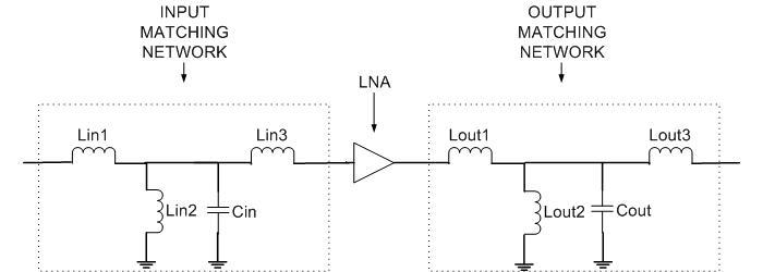
Figure 2: Matching network topology

The topology chosen, as seen in Figure 2, is a direct-coupled prototype bandpass network of parallel resonator type with top coupling [2], that is initially tuned to the geometric mean frequency with respect to the bandwidth of operation.

N = 3;                 % Order of input/output matching network
wU = 2*pi*fUpper;      % Upper band edge
wL = 2*pi*fLower;      % Lower band edge
w0 = sqrt(wL*wU);      % Geometric mean

For the initial design all the inductors are assigned the same value on the basis of the first series inductor. As mentioned in [3], choose the prototype value to be unity and use standard impedance and frequency transformations to obtain denormalized values [1]. The value for the capacitor in the parallel trap is set using this inductor value to make it resonate at the geometric mean frequency. Note that there are many ways of designing the initial matching network. This example shows one possible approach.

LvaluesIn = (Zs/(wU-wL))*ones(N,1);          % Series and shunt L's [H]
CvaluesIn = 1 / ( (w0^2)*LvaluesIn(2));      % Shunt C [F]
LvaluesOut = LvaluesIn;
CvaluesOut = CvaluesIn;

Build Matching Networks

Build each branch of the matching network and then define the circuit as a two-port network. This example uses identical input and output matching networks.

InputMatchingNW = circuit;
add(InputMatchingNW,[1 2],inductor(LvaluesIn(1)));
add(InputMatchingNW,[2 0],inductor(LvaluesIn(2)));
add(InputMatchingNW,[2 0],capacitor(CvaluesIn));
add(InputMatchingNW,[2 3],inductor(LvaluesIn(3)));
setports(InputMatchingNW,[1 0],[3 0]);

OutputMatchingNW = circuit;
add(OutputMatchingNW,[1 2],inductor(LvaluesOut(1)));
add(OutputMatchingNW,[2 0],inductor(LvaluesOut(2)));
add(OutputMatchingNW,[2 0],capacitor(CvaluesOut));
add(OutputMatchingNW,[2 3],inductor(LvaluesOut(3)));
setports(OutputMatchingNW,[1 0],[3 0]);

Optimize Input & Output Matching Network

There are several points to consider prior to the optimization.

Objective function: The objective function can be built in different ways depending on the problem at hand. For this example, the objective function is shown in the file below.
Choice of cost function: The cost function is the function you would like to minimize (maximize) to achieve near optimal performance. There could be several ways to choose the cost function. For this example you have two requirements to satisfy simultaneously, i.e. gain and noise figure. To create the cost function you first, find the difference, between the most current optimized network and the target value for each requirement at each frequency. The cost function is the L2-norm of the vector of gain and noise figure error values.
Optimization variables: In this case it is a vector of values, for the specific elements to optimize in the matching network.
Optimization method: A direct search based technique, the MATLAB® function fminsearch, is used in this example to perform the optimization.
Number of iterations/function evaluations: Set the maximum no. of iterations and function evaluations to perform, so as to tradeoff between speed and quality of match.
Tolerance value: Specify the variation in objective function value at which the optimization process should terminate.

The objective function used during the optimization process by fminsearch is shown here.

type('broadband_match_amplifier_objective_function.m')

function output = broadband_match_amplifier_objective_function(AMP,inMNW,outMNW,LC_Optim,freq,Gt_target,NF)
%BROADBAND_MATCH_AMPLIFIER_OBJECTIVE_FUNCTION is the objective function.
% OUTPUT = BROADBAND_MATCH_AMPLIFIER_OBJECTIVE_FUNCTION(AMP,INMNW,OUTMNW,LC_OPTIM,FREQ,GT_TARGET,NF) 
% returns the current value of the objective function stored in OUTPUT
% evaluated after updating the element values in the object, inMNW and 
% outMNW. The inductor and capacitor values are stored in the variable 
% LC_OPTIM.
%
% BROADBAND_MATCH_AMPLIFIER_OBJECTIVE_FUNCTION is an objective function of RF Toolbox demo:
% Designing Broadband Matching Networks (Part II: Amplifier)
 
%   Copyright 2023 The MathWorks, Inc.

% Ensure positive element values
if any(LC_Optim<=0)
    output = inf;
    return;
end
% Update matching network elements - The object inMNW and outMNW have 
% several properties among which the cell array 'Elements' consists of all 
% LC elements in the circuit.
inMNW.Elements(1).Inductance = LC_Optim(1);
inMNW.Elements(2).Inductance = LC_Optim(2);
inMNW.Elements(4).Inductance = LC_Optim(3);
inMNW.Elements(3).Capacitance = LC_Optim(4);
outMNW.Elements(1).Inductance = LC_Optim(5);
outMNW.Elements(2).Inductance = LC_Optim(6);
outMNW.Elements(4).Inductance = LC_Optim(7);
outMNW.Elements(3).Capacitance = LC_Optim(8);

% Perform analysis on tuned matching network
Npts           = length(freq);
BW             = max(freq) - min(freq);
np1            = nport(sparameters(inMNW,freq));
np2            = nport(sparameters(outMNW,freq));
b              = rfbudget([np1 clone(AMP) np2],freq',-30,BW);

% Calculate transducer power gains and noise figures of the amplifier
Gt             = b.TransducerGain(:,end);
NF_amp         = b.NF(:,end);

% Calculate target gain and noise figure error
errGt          = (Gt - Gt_target);
errNF          = (NF_amp - NF);

% Check to see if gain and noise figure target are achieved by specifying
% bounds for variation.
deltaG         = 0.40;
deltaNF        = -0.05;
errGt(abs(errGt)<=deltaG) = 0;
errNF(errNF<deltaNF) = 0;

% Cost function
err_vec        = [errGt;errNF];
output         = norm((err_vec),2);

% Animate
Gmax           = (Gt_target + deltaG).*ones(1,Npts);
Gmin           = (Gt_target - deltaG).*ones(1,Npts);
plot(freq*1e-6,Gt)
hold on
plot(freq*1e-6,NF_amp)
plot(freq.*1e-6,Gmax,'r-*')
plot(freq.*1e-6,Gmin,'r-*')
legend('G_t','NF','Gain bounds','Location','East');
xlabel('Freq [MHz]')
ylabel('Magnitude [dB]')
axis([freq(1)*1e-6 freq(end)*1e-6 0 Gt_target+2]);
hold off
drawnow;

The optimization variables are all the elements (inductors and capacitors) of the input and output matching networks.

nIter = 125; % Max No of Iterations
options = optimset('Display','iter','TolFun',1e-2,'MaxIter',nIter);   % Set options structure
LC_Optimized = [LvaluesIn;CvaluesIn;LvaluesOut;CvaluesOut];
LC_Optimized = fminsearch(@(LC_Optimized) broadband_match_amplifier_objective_function(Mismatched_Amp,InputMatchingNW,...
                             OutputMatchingNW,LC_Optimized,freq,Gt_target,NFtarget),LC_Optimized,options);

 
 Iteration   Func-count         f(x)         Procedure
     0            1          30.4869         
     1            9          28.3549         initial simplex
     2           11          25.5302         expand
     3           12          25.5302         reflect
     4           13          25.5302         reflect
     5           14          25.5302         reflect
     6           16          22.8228         expand
     7           17          22.8228         reflect
     8           19          19.0289         expand
     9           20          19.0289         reflect
    10           21          19.0289         reflect
    11           22          19.0289         reflect
    12           24          14.8785         expand
    13           25          14.8785         reflect
    14           27           10.721         expand
    15           28           10.721         reflect
    16           29           10.721         reflect
    17           31          9.84796         expand
    18           32          9.84796         reflect
    19           33          9.84796         reflect
    20           34          9.84796         reflect
    21           35          9.84796         reflect
    22           37          9.84796         contract outside
    23           39          9.84796         contract outside
    24           41          9.84796         contract inside
    25           43          9.64666         reflect
    26           45          9.64666         contract inside
    27           46          9.64666         reflect
    28           48          9.64666         contract inside
    29           49          9.64666         reflect
    30           51          9.64666         contract inside
    31           53           7.9372         expand
    32           55           7.9372         contract outside
    33           56           7.9372         reflect
    34           57           7.9372         reflect
    35           58           7.9372         reflect
    36           59           7.9372         reflect
    37           60           7.9372         reflect
    38           62          5.98211         expand
    39           63          5.98211         reflect
    40           64          5.98211         reflect
    41           65          5.98211         reflect
    42           66          5.98211         reflect
    43           68          4.31973         expand
    44           70          4.31973         contract inside
    45           71          4.31973         reflect
    46           72          4.31973         reflect
    47           73          4.31973         reflect
    48           74          4.31973         reflect
    49           75          4.31973         reflect
    50           77          2.83135         expand
    51           79          1.17624         expand
    52           80          1.17624         reflect
    53           81          1.17624         reflect
    54           82          1.17624         reflect
    55           84         0.691645         reflect
    56           85         0.691645         reflect
    57           86         0.691645         reflect
    58           88         0.691645         contract inside
    59           90         0.691645         contract outside
    60           91         0.691645         reflect
    61           93         0.691645         contract inside
    62           95         0.691645         contract inside
    63           96         0.691645         reflect
    64           97         0.691645         reflect
    65           98         0.691645         reflect
    66          100         0.691645         contract inside
    67          102         0.691645         contract outside
    68          103         0.691645         reflect
    69          105         0.691645         contract inside
    70          107         0.497434         reflect
    71          109         0.497434         contract inside
    72          111         0.497434         contract inside
    73          112         0.497434         reflect
    74          114         0.497434         contract inside
    75          116         0.497434         contract inside
    76          118         0.444957         reflect
    77          120         0.402851         expand
    78          122                0         reflect
    79          123                0         reflect
    80          125                0         contract inside
    81          127                0         contract inside
    82          128                0         reflect
    83          129                0         reflect
    84          130                0         reflect
    85          131                0         reflect
    86          132                0         reflect
    87          133                0         reflect
    88          134                0         reflect
    89          135                0         reflect
    90          137                0         contract inside

Figure contains an axes object. The axes object with xlabel Freq [MHz], ylabel Magnitude [dB] contains 4 objects of type line. These objects represent G_t, NF, Gain bounds.

    91          139                0         contract outside
 
Optimization terminated:
 the current x satisfies the termination criteria using OPTIONS.TolX of 1.000000e-04 
 and F(X) satisfies the convergence criteria using OPTIONS.TolFun of 1.000000e-02

Update Matching Network and Analyze LNA

Update the input and output matching networks with optimized element values, LC_Optimized.

InputMatchingNW.Elements(1).Inductance = LC_Optimized(1);
InputMatchingNW.Elements(2).Inductance = LC_Optimized(2);
InputMatchingNW.Elements(4).Inductance = LC_Optimized(3);
InputMatchingNW.Elements(3).Capacitance = LC_Optimized(4);
OutputMatchingNW.Elements(1).Inductance = LC_Optimized(5);
OutputMatchingNW.Elements(2).Inductance = LC_Optimized(6);
OutputMatchingNW.Elements(4).Inductance = LC_Optimized(7);
OutputMatchingNW.Elements(3).Capacitance = LC_Optimized(8);

Analyze the S-parameters of input and output matching networks and then convert the S-parameter data into an nport object.

s1 = sparameters(InputMatchingNW,freq);
np1 = nport(s1);
s2 = sparameters(OutputMatchingNW,freq);
np2 = nport(s2);

Use the rfbudget object to calculate the transducer gain and the noise figure across the bandwidth. Compute RF budget of the LNA network. The LNA network comprises of matching network and low noise amplifier.

bMatched = rfbudget([np1 clone(Mismatched_Amp) np2],freq',-30,BW);

Verify Design

Plot the transducer gain and the noise figure and then compare the optimization results with the mismatched network.

plot(freq*1e-6,bMatched.TransducerGain(:,end))
hold all
plot(freq*1e-6,bMismatched.TransducerGain(:,end))
plot(freq*1e-6,bMatched.NF(:,end))
plot(freq*1e-6,bMismatched.NF(:,end))
legend('G_t - Matched','G_t - Mismatched','NF - Matched',...
       'NF - Mismatched','Location','East')
xlabel('Frequency [MHz]')
ylabel('Magnitude [dB]')
axis([freq(1)*1e-6 freq(end)*1e-6 0 12])
grid on
hold off

Figure contains an axes object. The axes object with xlabel Frequency [MHz], ylabel Magnitude [dB] contains 4 objects of type line. These objects represent G_t - Matched, G_t - Mismatched, NF - Matched, NF - Mismatched.

The plot shows that the target requirement for both gain and noise figure have been met. To understand the effect of optimizing with respect to only the transducer gain, use the first choice for the cost function. The cost function involves only the gain term within the objective function.

Display Optimized Element Values

Display the optimized inductor and capacitor values for the input matching network.

Lin_Optimized = LC_Optimized(1:3)

Lin_Optimized = 3×1
10^-7 ×

    0.5722
    0.9272
    0.3546

Cin_Optimized = LC_Optimized(4)

Cin_Optimized = 6.8526e-12

Display the optimized inductor and capacitor values for the output matching network

Lout_Optimized = LC_Optimized(5:7)

Lout_Optimized = 3×1
10^-6 ×

    0.0517
    0.1275
    0.0581

Cout_Optimized = LC_Optimized(8)

Cout_Optimized = 5.4408e-12

Matching Network with Real-world Lumped Component Models

The real-world lumped components are selected from the Modelithics Select+ Library [5]. You must have the Modelithics Select+ Library license to run the following codes. Note that the Modelithics® LC elements are scaled with respect to the substrate characteristics. This example shows one possible approach using a 59 mil FR4 substrate.

Create RF Component from Modelithics SELECT+ Library

Set up the Modelithics Select+ Library by specifying the full path to the library.

mdlxSetup('C:\mdlx_library\SELECT')

Create the Modelithics® library object.

mdlx = mdlxLibrary;

Search the library for inductors with the optimized value for the input matching network.

search(mdlx,'FR4Standard59mil',Type='Inductors',Value=Lin_Optimized(1))

Search the library for capacitors with the optimized value for the input matching network.

search(mdlx,'FR4Standard59mil',Type='Capacitors',Value=Cin_Optimized)

Create an array of Modelithics® LC elements for the input and output matching networks.

Lin1_mdlx = search(mdlx,'FR4Standard59mil',Type='Inductors',Value=Lin_Optimized(1));
Lin2_mdlx = search(mdlx,'FR4Standard59mil',Type='Inductors',Value=Lin_Optimized(2));
Lin3_mdlx = search(mdlx,'FR4Standard59mil',Type='Inductors',Value=Lin_Optimized(3));
Cin_mdlx = search(mdlx,'FR4Standard59mil',Type='Capacitors',Value=Cin_Optimized);

Lout1_mdlx = search(mdlx,'FR4Standard59mil',Type='Inductors',Value=Lout_Optimized(1));
Lout2_mdlx = search(mdlx,'FR4Standard59mil',Type='Inductors',Value=Lout_Optimized(2));
Lout3_mdlx = search(mdlx,'FR4Standard59mil',Type='Inductors',Value=Lout_Optimized(3));
Cout_mdlx = search(mdlx,'FR4Standard59mil',Type='Capacitors',Value=Cout_Optimized);

Create and Anlyze Matching Networks

Create the input and output matching networks with Modelithics® capacitors and inductors. Note that most of the Modelithics® lumped components have two ports. Use the setports function to define the circuit as a 2-port network.

InputMatchingNWMdlx = circuit;
add(InputMatchingNWMdlx,[1 2 0 0],Lin1_mdlx(1));
add(InputMatchingNWMdlx,[2 0 0 0],Lin2_mdlx(1));
add(InputMatchingNWMdlx,[2 0 0 0],Cin_mdlx(1));
add(InputMatchingNWMdlx,[2 3 0 0],Lin3_mdlx(1));
setports(InputMatchingNWMdlx,[1 0],[3 0]);

OutputMatchingNWMdlx = circuit;
add(OutputMatchingNWMdlx,[1 2 0 0],Lout1_mdlx(1));
add(OutputMatchingNWMdlx,[2 0 0 0],Lout2_mdlx(1));
add(OutputMatchingNWMdlx,[2 0 0 0],Cout_mdlx(1));
add(OutputMatchingNWMdlx,[2 3 0 0],Lout3_mdlx(1));
setports(OutputMatchingNWMdlx,[1 0],[3 0]);

Analyze the S-parameters of input and output matching networks and then convert the S-parameter data into an nport object.

sm1 = sparameters(InputMatchingNWMdlx,freq);
npm1 = nport(sm1);

sm2 = sparameters(OutputMatchingNWMdlx,freq);
npm2 = nport(sm2);

bMatchedMdlx = rfbudget([npm1 clone(Mismatched_Amp) npm2],freq',-30,BW);

Verify Design

Plot the transducer gain and the noise figure of the real-world matching network and then compare the optimization results with the mismatched network.

figure
plot(freq*1e-6,bMatchedMdlx.TransducerGain(:,end))
hold all
plot(freq*1e-6,bMatched.TransducerGain(:,end))
plot(freq*1e-6,bMismatched.TransducerGain(:,end))
plot(freq*1e-6,bMatchedMdlx.NF(:,end))
plot(freq*1e-6,bMatched.NF(:,end))
plot(freq*1e-6,bMismatched.NF(:,end))
axis([freq(1)*1e-6 freq(end)*1e-6 0 12])
legend('G_t - Matched w/ Modelithics®','G_t - Matched w/ ideal',...
    'G_t - Mismatched','NF - Matched w/ Modelithics®','NF - Matched w/ ideal',...
       'NF - Mismatched','Position', [0.22643,0.47762,0.49643,0.25119])
xlabel('Frequency [MHz]')
ylabel('Magnitude [dB]')
grid on
hold off

The most noticeable aspect of the matching performance when using the Modelithics® library is the large deviation in transducer gain especially beyond 275 MHz. The noise figure performance has also worsened by approximately 0.25 dB. This can be explained by the fact that the inductor and capacitor models now represent real-world parasitic effects such as those due to the presence of a substrate, pads and orientation. This analysis highlights the importance of being able to predict such behaviors prior to realization of the design in hardware.

References

[1] Ludwig, Reinhold, and Gene Bogdanov. RF Circuit Design: Theory and Applications. Upper Saddle River, NJ: Prentice-Hall, 2009.

[2] Cuthbert, Thomas R. Broadband Direct-Coupled and Matching RF Networks. Greenwood, Ark.: T.R. Cuthbert, 1999.

[3] Cuthbert, T.R. “A Real Frequency Technique Optimizing Broadband Equalizer Elements.” In 2000 IEEE International Symposium on Circuits and Systems. Emerging Technologies for the 21st Century. Proceedings (IEEE Cat No.00CH36353), 5:401–4. Geneva, Switzerland: Presses Polytech. Univ. Romandes, 2000. https://doi.org/10.1109/ISCAS.2000.857453.

[4] Pozar, David M. Microwave Engineering. 4th ed. Hoboken, NJ: Wiley, 2012.

[5] https://www.modelithics.com/model/freemodels