4-Port Coupler in Shielded Enclosure

This example shows how to design and analyze a 4-Port coupler with a shielded enclosure. PCBs often experience unwanted problems such as electromagnetic interference (EMI) leading to performance degradation and failure. It may also affect other sensitive electronics due to outgoing EMI. An ideal shield will completely block off the EMI and ensure that strong signals cannot escape. Here you enclose a branchline coupler in a Faraday shield and analyze the coupler at 3 GHz using Finite Element Method (FEM).

Prerequisites

The example requires the Integro-Differential Modeling Framework for MATLAB add-on. To enable the add-on:

1. In the Home tab Environment section, click on Add-Ons. This opens the add-on explorer. You need an active internet connection to download the add-on.

2. Search for Integro-Differential Modeling Framework for MATLAB and click Install

3. To verify if the download is successful, run matlab.addons.installedAddons in your MATLAB® session command line.

Create Variables

Create variables for center frequency and frequency range.

Centerfreq = 3e9;
freq = linspace(1e9,5e9,40);

Design of Branchline Coupler

Use the design function to create a branchline coupler at the desired frequency. Visualize the coupler. The default substrate for a branchline coupler is Teflon.

branchline = couplerBranchline;
branchline = design(branchline,Centerfreq);
figure
show(branchline)

Use the sparameters function to compute the S-parameters from 1 GHz - 5 GHz. Plot the S-parameters.

spar1 = sparameters(branchline,freq);
figure
rfplot(spar1,1);
legend(Location="southwest")

S11 shows a good match around 2.8 GHz with a value less than -25 dB. The power is equally divided between Port 2 and Port 4, while Port 3 is isolated.

Plot the phase at the output ports, S21 and S41.

figure
rfplot(spar1,[2 4],1,'angle')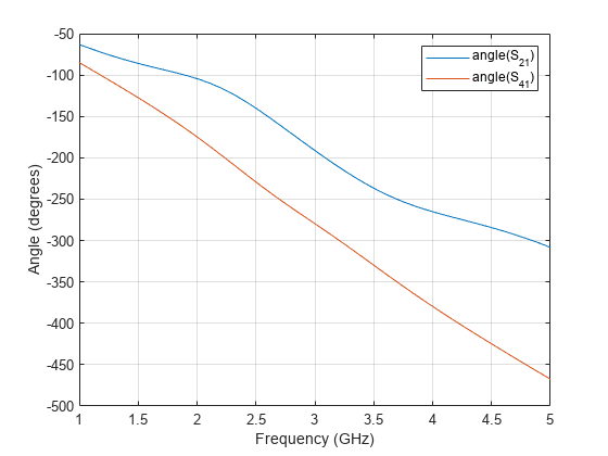

The result shows a 90 degree phase difference between output ports around 2.8 GHz.

Add Metal Shield

Add a 43 mm-by-53.8 mm-by-20 mm PEC shielded box to the branchline couple. View the coupler with the shield. You will see that the shield covers all four sides of the coupler. Move the shield in z-direction to align its bottom to the ground plane. The coupler is excited using a coaxial wave port with a default characteristic impedance of 50 ohms derived from outer or inner diameter and the dielectric constant of a coaxial.

branchline.IsShielded = true;
branchline.Shielding.Height = 0.02;
branchline.Shielding.Center = [0 0 0.5*branchline.Shielding.Height];
figure
show(branchline)

Display the layout of the branchline coupler. Add additional metals tapering out from the coaxial wave port with a width equal to coaxial inner diameter to the trace of a branchline coupler. The shape and length of added metal where a pin from a coaxial can sit on are determined by the PinFootprint and PinLength properties in Connector. This enables to examine a match between the coaxial and the board.

figure
layout(branchline)

Perform S-parameters Frequency Sweep

Use the sparameters function to compute the S-parameters of the shielded branchline coupler with added tapered metals at a frequency range of 1 GHz to 5 GHz.. Plot the S-parameters..

spar2 = sparameters(branchline,freq);
figure
rfplot(spar2,1)
legend(Location="southwest")
ylim([-30 0]);

Plot shows a general trend similar to that of the branchline coupler without a shielded box except there is a box resonance around 4.38 GHz.

Plot the phase of the output ports that are S21 and S41.

figure
rfplot(spar2,[2 4],1,'angle')

The result also shows a phase difference between output ports with a shielded box is 90 degrees around 2.8 GHz. A shielded box must be carefully designed otherwise the box resonances can result in unwanted performance at operating frequency.