Generate Code for Inverse Kinematics Computation Using Robot from Robot Library
This example shows how to perform code generation to compute Inverse Kinematics (IK) using robots from the robot library. For this example, you can use an inverseKinematics object with an included rigidBodyTree robot model using loadrobot to solve for robot configurations that achieve a desired end-effector position.
A circular trajectory is created in a 2-D plane and given as points to the generated MEX inverse kinematics solver. The solver computes the required joint positions to achieve this trajectory. Finally, the robot is animated to show the robot configurations that achieve the circular trajectory.
Write Algorithm to Solve Inverse Kinematics
Create a function, ikCodegen, that runs the inverse kinematics algorithm for a Kinova® Gen3 robot model created using loadrobot.
function qConfig = ikCodegen(endEffectorName,tform,weights,initialGuess)
    %#codegen
    persistent ik robot
    if isempty(robot)
        robot = loadrobot("kinovaGen3","DataFormat","row");
    end
    if isempty(ik)
        ik = inverseKinematics('RigidBodyTree',robot);
    end

    [qConfig,~] = ik(endEffectorName,tform,weights,initialGuess);
end
The algorithm acts as a wrapper for a standard inverse kinematics call. It loads the robot inside the function, accepts standard inputs, and returns a robot configuration solution vector. Since you cannot use handle objects as the input or output for functions that are supported for code generation. By setting them as persistent variables, the constructors used in this function are only called once. Without persistence, the mexed solver will be significantly slower.
Save the ikCodegen function in your current folder.
Verify Inverse Kinematics Algorithm in MATLAB
Verify the IK algorithm in MATLAB® before generating code.
Load a predefined Kinova® Gen3 robot model as rigidBodyTree object. Set the data format to "row".
robot = loadrobot("kinovaGen3",DataFormat="row");
Show details of the robot.
showdetails(robot)
--------------------
Robot: (8 bodies)

 Idx               Body Name         Joint Name         Joint Type               Parent Name(Idx)   Children Name(s)
 ---               ---------         ----------         ----------               ----------------   ----------------
   1           Shoulder_Link          Actuator1           revolute                   base_link(0)   HalfArm1_Link(2)
   2           HalfArm1_Link          Actuator2           revolute               Shoulder_Link(1)   HalfArm2_Link(3)
   3           HalfArm2_Link          Actuator3           revolute               HalfArm1_Link(2)   ForeArm_Link(4)
   4            ForeArm_Link          Actuator4           revolute               HalfArm2_Link(3)   Wrist1_Link(5)
   5             Wrist1_Link          Actuator5           revolute                ForeArm_Link(4)   Wrist2_Link(6)
   6             Wrist2_Link          Actuator6           revolute                 Wrist1_Link(5)   Bracelet_Link(7)
   7           Bracelet_Link          Actuator7           revolute                 Wrist2_Link(6)   EndEffector_Link(8)
   8        EndEffector_Link        Endeffector              fixed               Bracelet_Link(7)
--------------------
Specify the end-effector name, the weights for the end-effector transformation, and the initial joint positions.
endEffectorName = "EndEffector_Link";
weights = [0.25 0.25 0.25 1 1 1];
initialGuess = [0 0 0 0 0 0 0];
Call the inverse kinematics solver function for the specified end-effector transformation.
targetPose = trvec2tform([0.35 -0.35 0]);
qConfig = ikCodegen(endEffectorName,targetPose,weights,initialGuess)
qConfig = 1×7

    1.3085    2.2000   -1.3011    1.0072   -1.1144    2.0500   -3.2313
Visualize the robot with the computed robot configuration solution.
figure;
show(robot,qConfig);
hold on
plotTransforms(tform2trvec(targetPose),tform2quat(targetPose),FrameSize=0.5);
axis([-0.1 0.7 -0.5 0.5 -0.3 0.5])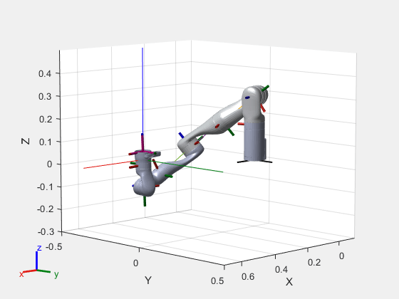
Generate Code for Inverse Kinematics Algorithm
You can use either the codegen (MATLAB Coder) function or the MATLAB Coder (MATLAB Coder) app to generate code. For this example, generate a MEX file by calling codegen at the MATLAB command line. Specify sample input arguments for each input to the function using the -args input argument.
Call the codegen function and specify the input arguments in a cell array. This function creates a separate ikCodegen_mex function to use. You can also produce C code by using the options input argument. This step can take some time.
codegen ikCodegen -args {endEffectorName,targetPose,weights,initialGuess}
Code generation successful.
Verify Results Using Generated MEX Function
Call the MEX version of the IK solver for the specified transform.
targetPose = trvec2tform([0.35 -0.35 0]);
qConfig = ikCodegen_mex(endEffectorName,targetPose,weights,initialGuess)
qConfig = 1×7

    1.3085    2.2000   -1.3011    1.0072    5.1688    2.0500   -3.2313
Visualize the robot with the robot configuration computed using the MEX version of the IK solver.
figure;
show(robot,qConfig);
hold on
plotTransforms(tform2trvec(targetPose),tform2quat(targetPose),FrameSize=0.5);
axis([-0.1 0.7 -0.5 0.5 -0.3 0.5])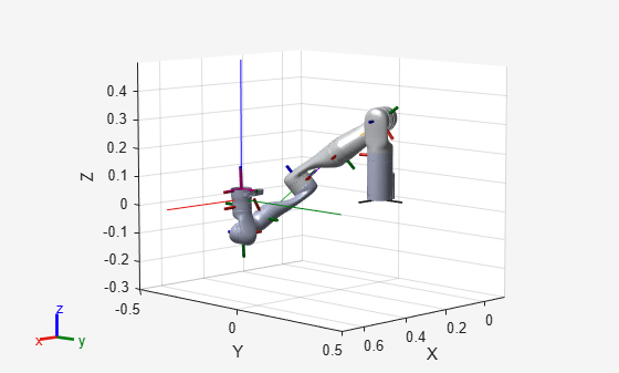
Compute Inverse Kinematics with MEX Function
Use the generated MEX function to compute the Inverse Kinematics solution to achieve a trajectory.
Define Trajectory
Create a circular trajectory.
t = (0:0.2:10)'; % Time
count = length(t);
center = [0.3 0.3 0];
radius = 0.15;
theta = t*(2*pi/t(end));
points = center + radius*[cos(theta) sin(theta) zeros(size(theta))];
Inverse Kinematics Solution
Preallocate configuration solutions as a matrix qs. Specify the weights for the end-effector transformation and the end-effector name.
q0 = [0 0 0 0 0 0 0];
ndof = length(q0);
qs = zeros(count,ndof);
weights = [0 0 0 1 1 1];
endEffector = "EndEffector_Link";
Loop through the trajectory of points to trace the circle. Use the ikCodegen_mex function to calculate the solution for each point to generate the joint configuration that achieves the end-effector position. Store the configurations for later use.
qInitial = q0; % Use home configuration as the initial guess
tic
for i = 1:count
    % Solve for the configuration satisfying the desired end-effector
    % position
    point = points(i,:);
    qSol = ikCodegen_mex(endEffector,trvec2tform(point),weights,qInitial);
    % Store the configuration
    qs(i,:) = qSol;
    % Start from prior solution
    qInitial = qSol;
end
loopTime = toc;
fprintf("Average (mexed) IK Execution Time: %f\n", loopTime/count);
Average (mexed) IK Execution Time: 0.001236
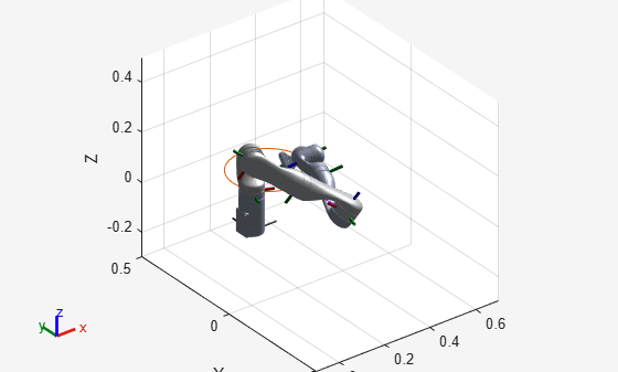
Animate Solution
Once you generate all the solutions, animate the results. You must recreate the robot because it was originally defined inside the function. Iterate through all the solutions. Set the "FastUpdate" option of the show method to true to get a smooth animation.
robot = loadrobot("kinovaGen3",DataFormat="row");
% Show first solution and set view.
figure
show(robot,qs(1,:));
view(3)
ax = gca;
ax.Projection = "orthographic";
hold on
plot(points(:,1),points(:,2))
axis([-0.1 0.7 -0.5 0.5 -0.3 0.5])

% Iterate through the solutions.
framesPerSecond = 15;
r = rateControl(framesPerSecond);
for i = 1:count
    show(robot,qs(i,:),PreservePlot=false,FastUpdate=true);
    drawnow
    waitfor(r);
end