Inverse Kinematics for Robots with Floating Base

Since R2024a

This example demonstrates how to solve the inverse kinematics problem for a robots modeled with a floating base. Floating-base robots can freely translate and rotate in space with six degrees of freedom. The inverse kinematics problem for floating-base robots is relevant in Space applications using a robotic arm, mounted on a floating and actuated base, to manipulate objects in Space, and for walking robots where the torso and legs are free to move in space.

Note that the rigidBodyTree object represents rigid body trees with a fixed base. That means that the base body of the rigid body tree has a fixed position and orientation in the world. You can attach a "floating" type rigid body joint to the base body to model robots with a floating base for some applications such as dynamic simulations. However, gradient-descent based inverse kinematics solvers, like the inverseKinematics function, do not support rigidBodyTree objects that contain "floating" type rigidBodyJoint joints. This is because the IK solver relies on the kinematic equation, $$Jq=\underset{}{\overset{\dot{}}{q}}$$, which relates the joint positions to instantaneous joint velocities of the robot using the geometric Jacobian. Given the number of columns of the Jacobian matrix are the velocity degrees of freedom, the number of position and velocity degrees of freedom must be equal for this equation to remain valid. Using a floating joint here would introduce a discrepancy because the floating joint uses a quaternion to represent rotation, which has four elements, while the corresponding angular velocity, has three elements. This example demonstrates how to model the floating base for use with the inverseKinematics function.

For more information about modeling a floating-base robot using the floating joint, see Model Floating-Base Robot Using Floating Joint.

Model Floating-Base Robot

To use the inverseKinematics solver for a floating-base robot, you must model a floating base rigid body and attach it to the fixed base of the robotic manipulator rigid body tree using six, consecutive one degree of freedom (DOF) joints. These six joints, consisting of three prismatic joints and three revolute joints, enable translation along and rotation about each of the x-, y-, and z-axes. In the home configuration, they are coincident with each other.

Load the rigid body model for the ABB IRB 120 to use as the robotic manipulator of the floating-base system.

abbirb = loadrobot("abbIrb120",DataFormat="row");

The helper function floatingBaseHelper creates a rigid body tree with six rigid bodies with no inertia or mass. The function connects each body in a series, and each is free to either translate or rotate about an axis in the world. The floatingBaseHelper creates a floating base as a rigid body tree that is both free to rotate and translate in the world with six degrees of freedom.

function robot = floatingBaseHelper(df)
    arguments
        df = "column"
    end
robot = rigidBodyTree(DataFormat=df);
robot.BaseName = 'world';
jointaxname = {'PX','PY','PZ','RX','RY','RZ'};
jointaxval = [eye(3); eye(3)];
parentname = robot.BaseName;
for i = 1:numel(jointaxname)
    bname = ['floating_base_',jointaxname{i}];
    jname = ['floating_base_',jointaxname{i}];
    rb = rigidBody(bname);
    rb.Mass = 0;
    rb.Inertia = zeros(1,6);
    rbjnt = rigidBodyJoint(jname,jointaxname{i}(1));
    rbjnt.JointAxis = jointaxval(i,:);
    rbjnt.PositionLimits = [-inf inf];
    rb.Joint = rbjnt;
    robot.addBody(rb,parentname);
    parentname = rb.Name;
end
end

Mount Robotic Arm onto Floating Base

Add the rigid body tree of the robotic arm abbirb to the floating base. Combined together into a floatingABBIrb, the system has a total of twelve degrees of freedom-six of the floating base and six (one for each revolute joint) of the original robotic arm.

floatingABBIrb = floatingBaseHelper("row");
addSubtree(floatingABBIrb,"floating_base_RZ",abbirb,ReplaceBase=false);

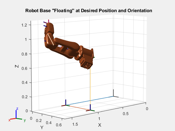
To demonstrate that the rigid body tree can both freely translate and rotate in space, visualize the base of the robotic arm at the xyz-coordinate [1.0 0.5 0.75], with an orientation [pi/4 pi/3 pi], and with zero joint angles of the robotic arm.

baseOrientation = [pi/4 pi/3 pi]; % ZYX Euler rotation order
basePosition = [1.0 0.5 0.75];
robotZeroConfig = zeros(1,6);
q = [basePosition baseOrientation zeros(1,6)];
show(floatingABBIrb,q);
axis equal;
title("Robot Base ''Floating'' at Desired Position and Orientation")

Solve Joint Configuration to Reach Target End-Effector Pose

In order to find the joint values for a given end-effector pose, use inverseKinematics function. Specify the end-effector body and the desired end-effector pose of the floating robotic arm.

eename = "tool0";
eepose = se3([0 pi/2 1.25],"eul",[-0.25 0.45 0.25]);

Create the inverseKinematics solver object to find the joint values corresponding to the desired eepose for the eename end-effector body on the floating rigid body tree. The weights are ones(1,6), specifying that solver should account for both the desired position and orientation of the end-effector. The initial guess for the joint configuration is the home configuration of the floating robotic arm.

ik = inverseKinematics(RigidBodyTree=floatingABBIrb);
[qsoln,solninfo] = ik(eename,eepose.tform,ones(1,6),homeConfiguration(floatingABBIrb));

Note that the pose error norm is very low and this means that the solution is sufficiently accurate.

disp(solninfo.Status)

success

Verify Joint Configuration

Plot the desired eepose and the solved joint configuration to visually verify that the end-effector frame aligns with the pose. Notice how the end-effector frame in this joint configuration is congruent to the desired eepose frame.

figure
plotTransforms(eepose,FrameSize=0.25,FrameLabel="eepose");
hold on
show(floatingABBIrb,qsoln);
hold off
axis equal
title("End Effector Reaches Desired Pose")

[v1,v2] = view

v1 = -37.5000

v2 = 30

The inverse kinematics solution enables the robot to achieve the desired end-effector pose, but because the rotation of the base is not constrained, the base can have any orientation. Display the orientation of the floating base in the solved joint configuration. Note that the floating base has a non-zero orientation.

disp(qsoln(4:6))

   -0.0005    0.2667   -0.2702

If the base is free to move, there are infinite solutions to the problem. If the base pose is known and the desired end-effector pose is reachable, it is possible to find a unique real joint configuration that satisfies the desired end-effector pose. Another approach is to constrain the base pose, by specifying constraints on the position and orientation depending on the requirements of your system. For example, in a gantry system that only permits translational movement of the base, you must constrain the orientation of the floating base.

Solving IK for Constrained Floating Base

To constrain the orientation of the floating base, set the JointPositionLimits property of the joints to limit the rotation about the x-, y-, and z-axes in the world frame to near zero. The inverse kinematics solver requires a small tolerance value of zero to avoid kinematic singularities. So instead of setting the joint limits to [0 0], set the joint limits to the smallest non-zero double precision values [-eps eps].

fb = getBody(floatingABBIrb,"floating_base_RX");
fb.Joint.PositionLimits = [-eps eps];
fb = getBody(floatingABBIrb,"floating_base_RY");
fb.Joint.PositionLimits = [-eps eps];
fb = getBody(floatingABBIrb,"floating_base_RZ");
fb.Joint.PositionLimits = [-eps eps];

Recreate the inverse kinematics solver for this rigid body tree and solve for the joint configuration.

ik = inverseKinematics(RigidBodyTree=floatingABBIrb);
[qsoln,solninfo] = ik(eename,eepose.tform,ones(1,6),homeConfiguration(floatingABBIrb));

Note that the inverse kinematics solver successfully found a joint configuration with almost no base orientation.

Display the success status of the solver and the orientation of the floating base.

disp(solninfo.Status)

success

disp(qsoln(4:6)) 

   1.0e-15 *

    0.2220    0.2220   -0.2220

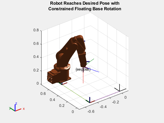
Visualize the joint configuration solution. Note that the robot reaches the desired pose while having a constrained floating base rotation.

figure
plotTransforms(eepose,FrameSize=0.25,FrameLabel="eepose");
hold on
show(floatingABBIrb,qsoln);
hold off
title(["Robot Reaches Desired Pose with","Constrained Floating Base Rotation"])
view([v1 v2])

Solving IK for Specified Base Pose

As stated earlier, there are infinite solutions to the IK problem for a floating-base system because the base can be anywhere and for every base pose there could exist a joint configuration of the robotic arm that satisfies an end-effector pose. Another approach, if the base pose is fixed and is known, is to solve for joint configurations given a specified base pose. Essentially treating the floating base as a fixed base.

First get the robotic arm subtree of the floating base system, starting from the original base of the robotic arm. Then create an IK solver for that subtree.

fixedBaseTree = subtree(floatingABBIrb,abbirb.BaseName);
ikFixedBaseTree = inverseKinematics("RigidBodyTree",fixedBaseTree);

Specify that the base is located at the xyz-position [-0.2 0.2 0.3] and at an orientation of [0.0 0.0 pi] Euler XYZ with respect to the world frame.

basePosition = [0.3 0.3 0.1];
baseEulXYZ = [0 0 pi]; %[-pi/4 0.0 -pi/3];

Since the inverseKinematics function computes joint values given an end-effector pose with respect to the fixed base of the rigid body tree, you must transform the end-effector pose eepose to the base frame before calculating the IK solution.

eePoseWrtFixedBase = se3(baseEulXYZ,"eul","XYZ",basePosition)\eepose;

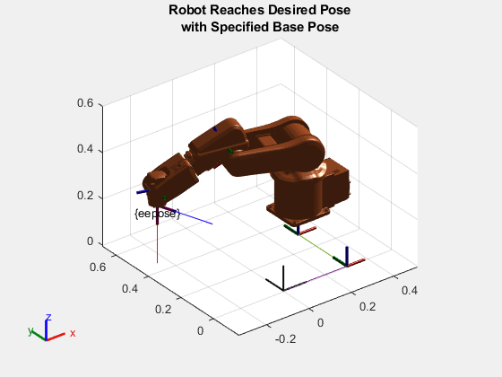
Visualize the joint positions qjoint in conjunction with the given fixed base position and base orientation to verify that the end-effector reaches the desired pose.

plotTransforms(eepose,FrameLabel="eepose",FrameSize=0.25);
hold on
[qjoint,solninfo] = ikFixedBaseTree(eename,eePoseWrtFixedBase.tform,ones(1,6),homeConfiguration(fixedBaseTree));
show(floatingABBIrb,[basePosition,baseEulXYZ,qjoint]);
title(["Robot Reaches Desired Pose","with Specified Base Pose"])
view([v1,v2])
hold off

Note that the IK solver was able to find a solution.

disp(solninfo.Status)

success