Threshold Parameter Tuning

This example shows how to compare values for the Follower power threshold parameter in the Simple Gear block for a basic mechanical system. Blocks like the Simple Gear block use threshold parameters to smoothly transition a physical characteristic between zero and nonzero. Threshold parameters like the Follower power threshold parameter in the Simple Gear block are a numerical tool that you can use to aid the solver with transition and improve simulation performance. The appropriate value for this parameter depends on the system. You must determine it on a case by case basis by comparing simulation step sizes for a range of values, but the same advice applies to all threshold parameters.

Run the Simulation

You can use the Follower power threshold parameter once you set Friction model to any setting other than No meshing losses - Suitable for HIL simulation. When you simulate meshing losses, the block uses the threshold parameter to transition between zero power transfer and partial power transfer. The script compares two different values for the threshold parameters while all else remains constant. To compare threshold parameter values, open the model:

mdl = "ThresholdParameterTuning";
open_system(mdl)

Run the simulation and record the data. Note that, in the output, only the first simulation generates warnings.

stop_time = 10;
out = run_sim(mdl, stop_time);

[05-Sep-2024 19:32:56] Running simulations...

Warning: Solver is encountering difficulty in simulating model 'ThresholdParameterTuning' at time 5.3597151906198555. Simulink will continue to simulate with warnings. Please check the model for errors.

Warning: Solver was unable to reduce the step size without violating minimum step size of 1.90415E-14 for 1 consecutive times at time 5.35972.  Solver will continue the simulation with the step size restricted to 1.90415E-14 and using an effective relative error tolerance of 0.0156906, which is greater than the specified relative error tolerance of 0.001. This usually may be caused by violating algebraic constraints in the differential-algebraic system or by the high stiffness of the system. Try tightening the error tolerances, and/or the tolerances for computing consistent conditions. If the problem persists, please check the system or increase the solver Number of consecutive min steps violation parameter. 
Suggested Actions:
    • Open Solver Profiler to explore such issues - Open

Warning: Solver is encountering difficulty in simulating model 'ThresholdParameterTuning' at time 5.3597151906198741. Simulink will continue to simulate with warnings. Please check the model for errors.

Warning: Solver was unable to reduce the step size without violating minimum step size of 1.90415E-14 for 2 consecutive times at time 5.35972.  Solver will continue the simulation with the step size restricted to 1.90415E-14 and using an effective relative error tolerance of 0.0313812, which is greater than the specified relative error tolerance of 0.001. This usually may be caused by violating algebraic constraints in the differential-algebraic system or by the high stiffness of the system. Try tightening the error tolerances, and/or the tolerances for computing consistent conditions. If the problem persists, please check the system or increase the solver Number of consecutive min steps violation parameter. 
Suggested Actions:
    • Open Solver Profiler to explore such issues - Open

Warning: Solver is encountering difficulty in simulating model 'ThresholdParameterTuning' at time 5.3597151906198928. Simulink will continue to simulate with warnings. Please check the model for errors.

Warning: Solver was unable to reduce the step size without violating minimum step size of 1.90415E-14 for 3 consecutive times at time 5.35972.  Solver will continue the simulation with the step size restricted to 1.90415E-14 and using an effective relative error tolerance of 0.0156906, which is greater than the specified relative error tolerance of 0.001. This usually may be caused by violating algebraic constraints in the differential-algebraic system or by the high stiffness of the system. Try tightening the error tolerances, and/or the tolerances for computing consistent conditions. If the problem persists, please check the system or increase the solver Number of consecutive min steps violation parameter. 
Suggested Actions:
    • Open Solver Profiler to explore such issues - Open

[05-Sep-2024 19:33:03] Completed 1 of 2 simulation runs
[05-Sep-2024 19:33:04] Completed 2 of 2 simulation runs

Plot the Results

Collect the logged data from the simulation runs.

data1 = collect_data(out(1));
data2 = collect_data(out(2));

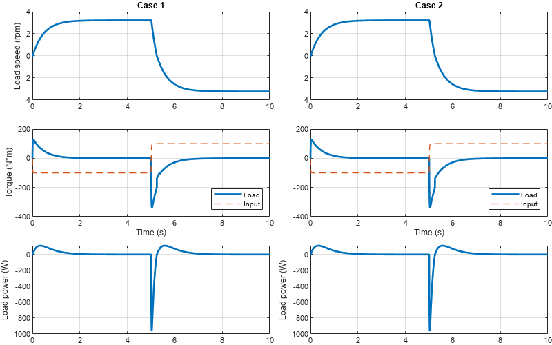
Make plots comparing physical quantities. The simulation data looks similar for both cases.

plot_result(data1, data2)

Compare Simulation Step Size

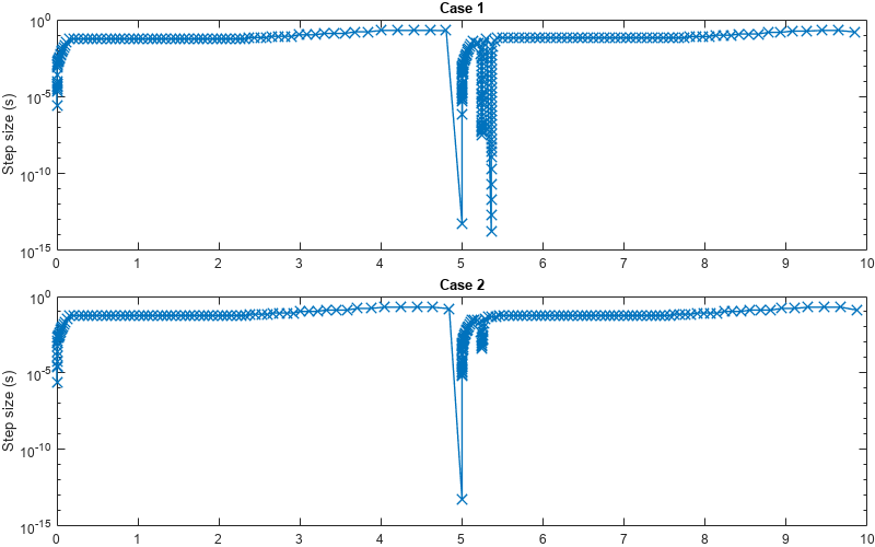
Despite the similarity in the simulation output, the performance is different for each case. Plot a comparison of the step size data. Note the difference at approximately five seconds.

plot_step_size([0 stop_time], data1, data2)

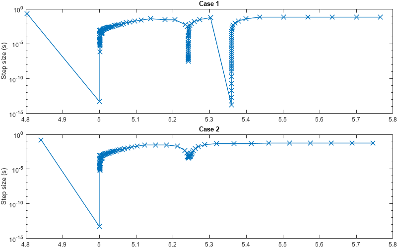
To get a better view of the results at approximately five seconds, zoom in on the plot.

plot_step_size([4.8 5.8], data1, data2)

In case 1, the value for the Follower power threshold parameter is 0.001 W. In case 2, the value is 10 W. When you plot the power of the load inertia, you can see that the power is in the range of about 1 W and 1000 W. A threshold value of 0.001 W is too small compared to the typical power range of the system while 10 W is roughly one percent of the total power range that the system can exhibit. A value that is too small makes it difficult for the solver to satisfy its error tolerances. The solver must take many small step sizes, which negatively impacts simulation performance.

function out = run_sim(mdl, stop_time)
load_system(mdl)

clear simin
simin(1:2) = Simulink.SimulationInput(mdl);

% Use variable step solver, DAE SSC.
simin = setModelParameter(simin, ...
  SolverType = "Variable-step", ...
  Solver = "daessc", ...
  StopTime = num2str(stop_time));

% Turn off the Simscape local solver.
simin = setBlockParameter(simin, mdl + "/Solver Configuration", ...
  UseLocalSolver = "off");

% Set two different values for Follower power threshold in Simple Gear block.
simin(1) = setBlockParameter(simin(1), mdl + "/Simple Gear", pwr_thr = "0.001");
simin(2) = setBlockParameter(simin(2), mdl + "/Simple Gear", pwr_thr = "10");

% Make sure to use the same unit for Follower power threshold.
simin = setBlockParameter(simin, mdl + "/Simple Gear", pwr_thr_unit = "W");

% Apply the final (second) settings to the model file.
applyToModel(simin(end))

% Run simulation. This runs 2 simulation cases as defined in simin.
out = sim(simin);
end
function data = collect_data(out)
data.source_time   = out.simlog_ThresholdParameterTuning.Torque_Source.S.series.time;
data.source_torque = out.simlog_ThresholdParameterTuning.Torque_Source.S.series.values("N*m");

data.input_speed  = out.simlog_ThresholdParameterTuning.Input_Inertia.w.series.values("rad/s");
data.input_torque = out.simlog_ThresholdParameterTuning.Input_Inertia.t.series.values("N*m");
data.input_power = data.input_speed .* data.input_torque;

data.load_time = out.simlog_ThresholdParameterTuning.Load_Inertia.w.series.time;
data.load_step_size = diff(data.load_time);
data.load_speed  = out.simlog_ThresholdParameterTuning.Load_Inertia.w.series.values("rad/s");
data.load_torque = out.simlog_ThresholdParameterTuning.Load_Inertia.t.series.values("N*m");
data.load_power = data.load_speed .* data.load_torque;
end

function plot_result(data1, data2)
fig = figure;
fig.Position(3:4) = [800 500];  % width height

layout = tiledlayout(fig, 3, 2);
layout.TileIndexing = "columnmajor";
layout.TileSpacing = "compact";
layout.Padding = "tight";

% left column

tile = nexttile(layout);
plot(tile, data1.load_time, data1.load_speed, LineWidth=2)
grid on
ylabel(tile, "Load speed (rpm)")
title(tile, "Case 1")

tile = nexttile(layout);
plot(tile, data1.load_time, data1.load_torque, LineWidth=2)
hold on
plot(tile, data1.source_time, data1.source_torque, LineWidth=1, LineStyle="--")
grid on
legend(tile, ["Load" "Input"], Location="southeast")
ylabel(tile, "Torque (N*m)")
xlabel(tile, "Time (s)")

tile = nexttile(layout);
plot(tile, data1.load_time, data1.load_power, LineWidth=2)
grid on
ylabel(tile, "Load power (W)")

% right column

tile = nexttile(layout);
plot(tile, data2.load_time, data2.load_speed, LineWidth=2)
grid on
title(tile, "Case 2")

tile = nexttile(layout);
plot(tile, data2.load_time, data2.load_torque, LineWidth=2)
hold on
plot(tile, data2.source_time, data2.source_torque, LineWidth=1, LineStyle="--")
grid on
legend(tile, ["Load" "Input"], Location="southeast")
xlabel(tile, "Time (s)")

tile = nexttile(layout);
plot(tile, data2.load_time, data2.load_power, LineWidth=2)
grid on
ylabel(tile, "Load power (W)")
end
function plot_step_size(time_range, data1, data2)
fig = figure;
fig.Position(3:4) = [800 500];  % width height

layout = tiledlayout(fig, 2, 1);
layout.TileIndexing = "columnmajor";
layout.TileSpacing = "compact";
layout.Padding = "tight";

tile = nexttile(layout);
logical_index = data1.load_time >= time_range(1) & data1.load_time < time_range(2);
p = semilogy(tile, data1.load_time(logical_index), data1.load_step_size(logical_index));
p.LineWidth = 1;
p.Marker = "x";
p.MarkerSize = 10;
xlim(time_range)
ylabel(tile, "Step size (s)")
title(tile, "Case 1")

tile = nexttile(layout);
logical_index = data2.load_time >= time_range(1) & data2.load_time < time_range(2);
p = semilogy(tile, data2.load_time(logical_index), data2.load_step_size(logical_index));
p.LineWidth = 1;
p.Marker = "x";
p.MarkerSize = 10;
xlim(time_range)
ylabel(tile, "Step size (s)")
title(tile, "Case 2")
end