La traduction de cette page n'est pas à jour. Cliquez ici pour voir la dernière version en anglais.

Graph Importer

Extraire des graphes depuis des fiches techniques afin de les utiliser dans le paramétrage des blocs

Depuis R2024a

Description

Utilisez l’outil Graph Importer pour importer des graphes depuis des fiches techniques de pièces, modifier les données de point si nécessaire, puis exporter les données sélectionnées sous la forme de fichiers de données MATLAB^®. Vous pouvez ensuite utiliser ces fichiers de données pour le paramétrage des blocs.

L’outil Graph Importer propose les fonctions suivantes :

Importer des graphes depuis des fiches techniques de pièces au format PDF.
Calibrer les axes de données.
Sélectionner les points pertinents sur les courbes de données et constituer une table.
Modifier éventuellement les données de point en déplaçant les points ou en apportant des modifications à la table.
Tracer éventuellement plusieurs courbes sur une grille commune le long de l’axe X.
Exporter les données sélectionnées sous la forme de fichiers de données MATLAB.

Ouvrir Graph Importer

À l’invite de commande MATLAB : saisissez graphImporter.

Exemples

développer tout

Extraire des points d’un tracé de fiche technique vers une table de données

Ouvrez une fiche technique du fabricant au format PDF. Au moyen de Microsoft^® Snipping Tool ou d’une application similaire, effectuez une capture du tracé qui vous intéresse et enregistrez-la dans un fichier image. Les formats de fichier supportés sont les suivants : bmp, gif, jpg, jpeg, png, tif.
Ouvrez Graph Importer :
```
graphImporter
```
Cliquez sur New Session et sélectionnez le fichier image enregistré à l’étape 1.
Suivez les invites de la fenêtre Graph Importer. Commencez par spécifier l’échelle du tracé en sélectionnant les points de référence sur les axes X et Y, et en saisissant les valeurs correspondantes dans les champs Toolstrip. Nul besoin de sélectionner de points minimum et maximum. Sélectionnez deux points de référence pour chaque axe : l’outil calibre alors le tracé sur la base des valeurs que vous saisissez.
Sélectionnez un point sur l’axe X. L’outil repère le point en lui attribuant la couleur verte.
Dans Graph Importer Toolstrip, saisissez 0.5 dans le champ X-axis first point.
Répétez l’opération pour le deuxième point de référence sur l’axe X. Sélectionnez ensuite deux points de référence sur l’axe Y et saisissez également les valeurs dans les champs Toolstrip.
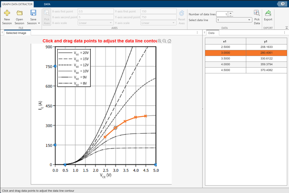
Dans cet exemple, vous allez importer des points à partir d’une ligne de données. Par conséquent, conservez la valeur Number of data lines à 1.
Activez le bouton Pick Data et sélectionnez plusieurs points sur la troisième ligne en partant du bas, qui correspond à V_CE = 10V.
L'outil repère les points sélectionnés en leur attribuant la couleur rouge et génère une table reprenant les coordonnées X et Y de chaque point.
Pour ajuster les positions des points, désactivez le bouton Pick Data. Faites glisser le deuxième point le long de la ligne jusqu'à x1 = 3.0000. Lorsque vous commencez à faire glisser un point, les cellules de la table correspondante sont mises en surbrillance en rouge. Vous pouvez saisir les coordonnées souhaitées directement dans les cellules de la table.
Lorsque les positions des points vous conviennent, cliquez sur Export et indiquez le nom du fichier, par exemple IGBT_plot1. L’outil exporte la table sous la forme d’un fichier MAT. Vous pouvez ensuite utiliser ce fichier pour le paramétrage des blocs.
Cliquez sur le bouton Save Session et enregistrez l’état actuel de l’outil Graph Importer sous la forme d’un fichier MAT. Pour le distinguer du fichier IGBT_plot1.mat qui contient uniquement les données d’exportation de la table, attribuez au fichier de la session enregistrée le nom IGBT_plot1_session1.mat. Plus tard, vous pourrez charger le fichier d’une session enregistrée dans Graph Importer et ajouter ou modifier des points de données, comme l’illustre l’exemple suivant.

Extraire plusieurs lignes d’une fiche technique et les tracer sur une grille

Ouvrez Graph Importer :
```
graphImporter
```
Cliquez sur Open Session et sélectionnez le fichier de session IGBT_plot1_session1.mat que vous avez enregistré dans le cadre de l’exemple précédent.
La table présentée dans le volet de droite de la fenêtre Graph Importer contient les coordonnées x1 et y1 des cinq points de données sélectionnés sur la ligne de tracé V_CE = 10V. Vous allez à présent ajouter des points issus d’une deuxième ligne.
Dans Toolstrip, définissez la valeur Number of data lines sur 2.
Dans la liste déroulante Select data line, sélectionnez 2.
Activez le bouton Pick Data et sélectionnez sept points sur la quatrième ligne en partant du bas, qui correspond à V_CE = 12V.
L’outil repère les points sélectionnés en leur attribuant la couleur violette et ajoute les colonnes x2 et y2 à la table. Ces colonnes contiennent les coordonnées X et Y de chaque point de la deuxième ligne.
Remarque : les points de la deuxième ligne sont au nombre de sept, tandis que la première n’en comporte que cinq. Par conséquent, la table contient des cellules vides (NaN) au bas des colonnes x1 et y1.
Pour tracer les deux lignes sur une grille le long de l’axe X, cliquez sur l’onglet Data dans Graph Importer Toolstrip.
Cliquez sur le bouton radio Gridded, puis cliquez sur Interpolate.
L'outil interpole les deux courbes entre les valeurs X minimum et maximum, chaque courbe comportant désormais sept points équidistants le long de l'axe X. La table de données ne contient désormais que trois colonnes : x (commune aux deux courbes), y1 et y2.
Remarque : si vous tentez d’ajuster les positions des points, vous ne pouvez plus que les déplacer le long de l'axe Y car la valeur X reste identique.
Les champs Toolstrip X-data minimum et X-data maximum indiquent la plage d’interpolation. Le champ Number of ticks indique le nombre de points de grille le long de l'axe X. Pour aligner les données sur la grille dans le tracé, définissez la valeur Number of ticks sur 5.
Une nouvelle fois, l’outil interpole les deux courbes, chaque courbe comportant désormais cinq points. La table des données contient cinq lignes de données.
Lorsque la table des données vous convient, cliquez sur Export et indiquez le nom du fichier, IGBT_plot2.

Exemples associés

Parameterizing Blocks from Datasheets (Simscape Electrical)

Utilisation programmatique

développer tout

`graphImporter`

graphImporter ouvre l’outil Graph Importer.

Historique des versions

Introduit dans R2024a