Digital Waveform Generation: Approximate a Sine Wave
This example shows how to design and evaluate a sine wave data table for use in digital waveform synthesis applications in embedded systems and arbitrary waveform generation instruments.
Even small systems use real-time direct digital synthesis of analog waveforms using embedded processors and digital signal processors (DSPs) connected to digital-to-analog converters (DACs). Using MATLAB® and Simulink®, you can develop and analyze the waveform generation algorithm and its associated data before implementing it with Simulink Coder™ on target hardware.
The most accurate way to digitally synthesize a sine wave is to compute the full-precision sin function directly for each time step, folding omega*t into the interval 0 to 2*pi. In real-time systems, the computational burden is typically too large for this approach. Alternatively, you can use a table of values to approximate the behavior of the sin function, either from 0 to 2*pi, half-wave, or quarter-wave data.
Tradeoffs between the two approaches include algorithm efficiency, data ROM size required, and the accuracy and spectral purity of the implementation. Similar analysis is needed when performing your own waveform designs. The table data and look-up algorithm alone do not determine performance in the field. Additional considerations, such as the accuracy and stability of the real-time clock and digital-to-analog conversion, are required to assess overall performance. The Signal Processing Toolbox™ and the DSP System Toolbox™ complement the capabilities of MATLAB and Simulink for work in this area.
Another method to approximate the behavior of the sine wave is to use the coordinate rotation digital computer (CORDIC) approximation. The Givens rotation-based CORDIC algorithm is one of the most hardware-efficient algorithms because it requires only shift-add iterative operations.
Create Table in Double Precision Floating Point
These commands make a 256-point sine wave and measure its total harmonic distortion when sampled first on the points and then by jumping with a delta of 2.5 points per step using linear interpolation. Similar computations are done by replacing the sine values with CORDIC sine approximation. For frequency-based applications, spectral purity can be more important than absolute error in the table.
In this example, the file ssinthd.m calculates the total harmonic distortion (THD) for digital sine wave generation with or without interpolation. This THD algorithm proceeds over an integral number of waves to achieve accurate results. The number of wave cycles used is A. The step size 'delta' is A/B. Traversing A waves hit all points in the table at least one time, which is needed to accurately find the average THD across a full cycle.
The relationship used to calculate THD is
THD = (ET - EF) / ET,
where ET = total energy and EF = fundamental energy.
The energy difference between ET and EF is spurious energy.
N = 256;
angle = 2*pi*(0:(N-1))/N;

s = sin(angle)';
thd_ref_1 = ssinthd(s,1,N,1,'direct' );
thd_ref_2p5 = ssinthd(s,5/2,2*N,5,'linear' );

cs = cordicsin(angle,50)';
thd_ref_1c = ssinthd(cs,1,N,1,'direct' );
thd_ref_2p5c = ssinthd(cs,5/2,2*N,5,'linear' );
Use Sine Wave Approximations in a Model
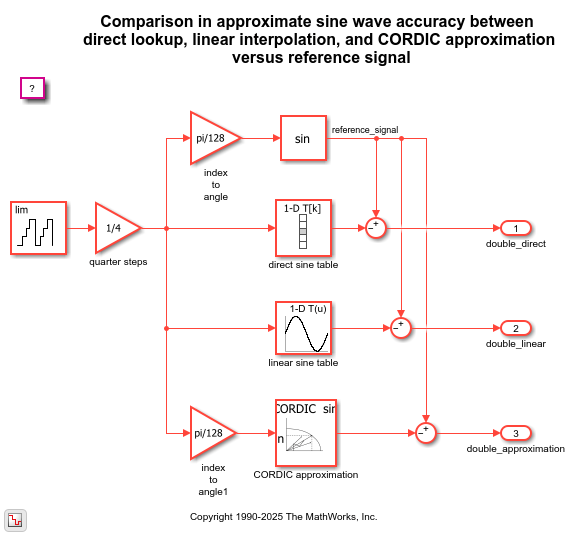
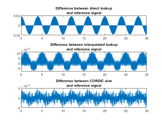
You can put the sine wave you design into a Simulink model and see how it works as a direct lookup with linear interpolation and with CORDIC approximation. This model compares the output of the floating-point tables to the sin function. As expected from the THD calculations, the linear interpolation has a lower error than the direct table lookup in comparison to the sin function. The CORDIC approximation shows a lower error margin when compared to the linear interpolation method. This margin depends on the number of iterations when computing the CORDIC sin approximation. You can typically achieve greater accuracy by increasing the number of iterations. The CORDIC approximation eliminates the need for explicit multipliers. This is used when multipliers are less efficient or non-existent in hardware.
Open and simulate the sldemo_tonegen model.
open_system('sldemo_tonegen');
set_param('sldemo_tonegen', 'StopFcn','');
out = sim('sldemo_tonegen');
Optionally, extract the simulation execution time from the timing information stored in Simulink.SimulationMetadata
runTime=out.SimulationMetadata.TimingInfo;
normalExec = runTime.ExecutionElapsedWallTime;
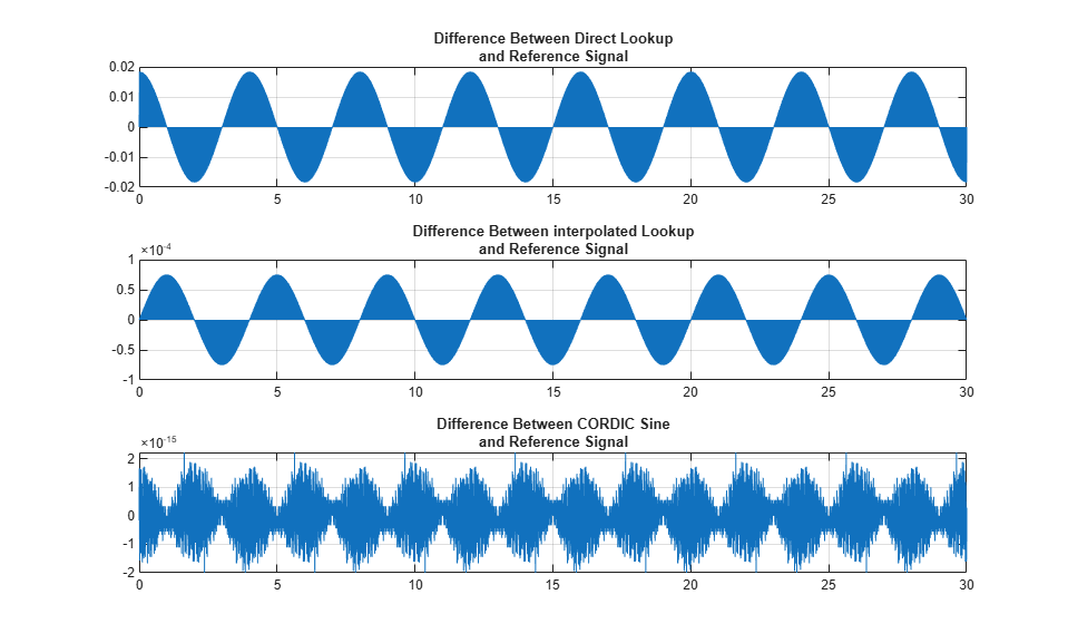
Plot the simulation output.
currentFig = figure('Color',[1,1,1]);
subplot(3,1,1), plot(out.tonegenOut.time, out.tonegenOut.signals(1).values); grid
title({'Difference Between Direct Lookup', 'and Reference Signal'});
subplot(3,1,2), plot(out.tonegenOut.time, out.tonegenOut.signals(2).values); grid
title({'Difference Between interpolated Lookup', 'and Reference Signal'});
subplot(3,1,3), plot(out.tonegenOut.time, out.tonegenOut.signals(3).values); grid
title({'Difference Between CORDIC Sine', 'and Reference Signal'});
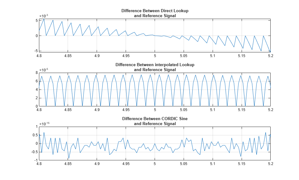
Examine Waveform Accuracy
When you examine signals, you can see different characteristics of the different algorithms. For example, zoom in on the signals between 4.5 and 5.2 seconds of simulation time.
ax = get(currentFig,'Children');
set(ax(3),'xlim',[4.8, 5.2]);
set(ax(2),'xlim',[4.8, 5.2]);
set(ax(1),'xlim',[4.8, 5.2]);
Implement Table in Fixed Point
You can convert the floating-point table into a 24-bit fractional number using nearest rounding. Test the new table for total harmonic distortion in direct lookup mode at 1, 2, and 3 points per step and then with fixed-point linear interpolation.
bits = 24;
is = num2fixpt(s,sfrac(bits),[],'Nearest','on');

thd_direct1 = ssinthd(is,1,N,1,'direct');
thd_direct2 = ssinthd(is,2,N,2,'direct');
thd_direct3 = ssinthd(is,3,N,3,'direct');

thd_linterp_2p5 = ssinthd(is,5/2,2*N,5,'fixptlinear');
Compare Results
Choosing a table step rate of 8.25 points per step (33/4), jump through the double-precision and fixed-point tables in direct and linear modes and compare distortion results.
thd_double_direct = ssinthd(s,33/4,4*N,33,'direct');
thd_sfrac24_direct= ssinthd(is,33/4,4*N,33,'direct');

thd_double_linear = ssinthd( s,33/4,4*N,33,'linear');
thd_sfrac24_linear = ssinthd(is,33/4,4*N,33,'fixptlinear');
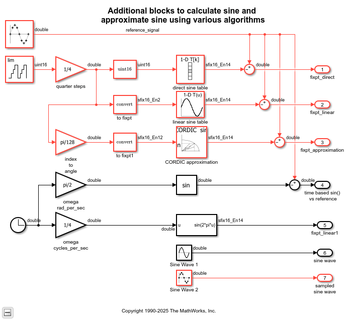
Use Preconfigured Sine Wave Blocks
Simulink also includes a Sine Wave block with continuous and discrete modes, plus fixed-point Sine and Cosine function blocks that implement the function approximation with a linearly interpolated lookup table that exploits the quarter wave symmetry of sine and cosine. The model sldemo_tonegen_fixpt uses a sampled sine wave source as the reference signal and compares it with a lookup table with or without interpolation, and with CORDIC sine approximation in fixed-point data types.
Open the sldemo_tonegen_fixpt model.
open_system('sldemo_tonegen_fixpt');
set_param('sldemo_tonegen_fixpt', 'StopFcn','');
out = sim('sldemo_tonegen_fixpt');
Optionally, extract the simulation execution time from the timing information stored in Simulink.SimulationMetadata.
runTime=out.SimulationMetadata.TimingInfo;
normalExec = runTime.ExecutionElapsedWallTime;
Plot the simulation output.
figure('Color',[1,1,1]);
subplot(3,1,1), plot(out.tonegenOut.time, out.tonegenOut.signals(1).values); grid
title({'Difference Between Direct Lookup', 'and Reference Signal'});
subplot(3,1,2), plot(out.tonegenOut.time, out.tonegenOut.signals(2).values); grid
title({'Difference Between Interpolated Lookup', 'and Reference Signal'});
subplot(3,1,3), plot(out.tonegenOut.time, out.tonegenOut.signals(3).values); grid
title({'Difference Between CORDIC Sine', 'and Reference Signal'});
Use Sine Function with Clock Input
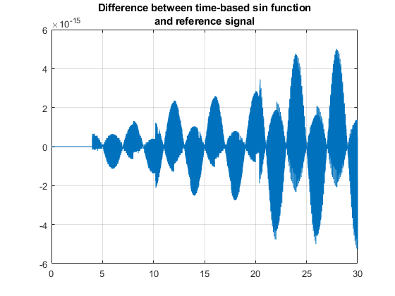
The model also compares the sine wave source reference with the sin function whose input angle in radians is time-based, or computed using a clock. You can test the assumption that the clock input would return repeatable results from the sin function for period 2*pi. This plot shows that the sin function accumulates error when its input is time-based. The plot also shows that a sampled sine wave source is more accurate to use as a waveform generator.
subplot(1,1,1), plot(out.tonegenOut.time, out.tonegenOut.signals(4).values); grid
title({'Difference Between Time-Based Sin Function', 'and Reference Signal'});
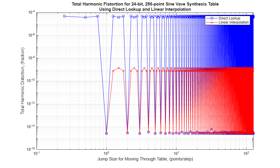
Survey of Behavior for Direct Lookup and Linear Interpolation
To perform a full-frequency sweep of the fixed-point tables and gain insight to the behavior of this design, run the file sldemo_sweeptable_thd.m. Total harmonic distortion of the 24-bit fractional fixed-point table is measured at each step size, and moves through D points at a time, where D is a number from 1 to N/2, incremented by 0.25 points. N is 256 points in this example. Frequency is discrete and therefore a function of the sample rate.
Notice the modes of the distortion behavior in the plot. When retrieving from the table precisely at a point, the error is smallest. Linear interpolation has a smaller error than direct lookup between points. However, the error is relatively constant for each of the modes up to the Nyquist frequency.
figure('Color',[1,1,1]);
sldemo_sweeptable_thd(24, 256)
Next Steps
Using CORDIC approximation, you can run this example using different numbers of iterations to see the effects on accuracy and computation time. Try different implementation options for waveform synthesis algorithms using automatic code generation available in Simulink Coder and production code generation using Embedded Coder®. Embedded target products offer direct connections to a variety of real-time processors and DSPs, including connection back to the Simulink model while the target is running in real-time. The Signal Processing Toolbox and DSP System Toolbox offer capabilities for designing and implementing a wide variety of sample-based and frame-based signal processing systems with MATLAB and Simulink.
References
[1] Chrysafis, Andrea. "Digital Sine-Wave Synthesis Using the DSP56001/2." Motorola, 1988.
See Also
Sine, Cosine | Sine Wave | Sine Wave Function | Simulink.SimulationMetadata
Topics
- Fixed-Point Math Operations in MATLAB and Simulink (Fixed-Point Designer)