Single Hydraulic Cylinder Simulation
This example shows how to use Simulink® to model a hydraulic cylinder. You can apply these concepts to applications where you need to model hydraulic behavior.
Model Analysis and Physics
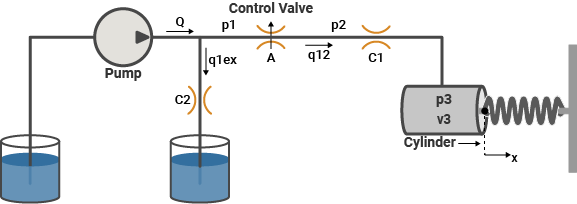
This schematic diagram shows a model of a hydraulic cylinder. The model directs the pump flow, Q, to supply pressure, p1, from which the laminar flow, q1ex, leaks to exhaust. The control valve for the piston/cylinder assembly is modeled as turbulent flow through a variable-area orifice. Its flow, q12, leads to intermediate pressure, p2, which undergoes a subsequent pressure drop in the line connecting it to the actuator cylinder. The cylinder pressure, p3, moves the piston against a spring load, resulting in position x.
At the pump output, the flow is split between leakage and flow to the control valve. The model uses the Equation Set 1 equations to simulate the leakage, q1ex, as laminar flow.
Equation Set 1


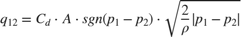
The model implements the orifice equation to simulate turbulent flow through the control valve. The sign and absolute value functions accommodate flow in either direction, as shown in Equation Set 2.
Equation Set 2


The fluid within the cylinder pressurizes due to the fluid flow, q12 = q23, minus the compliance of the piston motion. The model implements the fluid flow and flow compressibility using the Equation Set 3 equations.
Equation Set 3
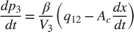


The model neglects the piston and spring masses because of the large hydraulic forces. The system of equations is incorporated by differentiating this relationship and incorporating the pressure drop between p2 and p3.
Equation Set 3 models laminar flow from the valve to the actuator. Equation Set 4 gives the force balance at the piston.
Equation Set 4


Run the Simulation
To run the simulation, on the Simulink Toolstrip, click Run.
During simulation, the model logs relevant data to the MATLAB workspace in the Simulink.SimulationOutput object out. Signal logging data is stored in the out object, in a structure called sldemo_hydcyl_output. Logged signals have a blue badge.

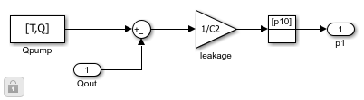
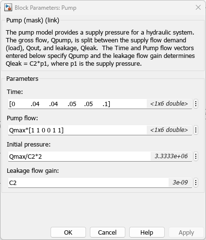
Pump Subsystem
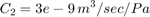
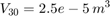
To look under the Pump subsystem mask, right-click the Pump subsystem and select Edit Mask > Look Under Mask. The pump model computes the supply pressure as a function of the pump flow and the load (output) flow. Qpump is the pump flow data, which is saved in the model workspace. A matrix with column vectors of time points and the corresponding flow rates [T,Q] specifies the flow data. The model calculates pressure p1, as indicated in Equation Set 1. Because Qout = q12 is a direct function of p1 via the control valve, an algebraic loop is formed. An estimate of the initial value, p10, enables a more efficient solution.
You can use 'Pump' subsystem mask to access and change the T, Q, p10, and C2 parameters.
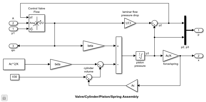
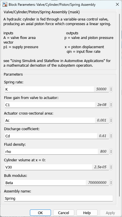
Valve/Cylinder/Piston/Spring Assembly Subsystem
To view the Actuator subsystem, right-click the masked Valve/Cylinder/Piston/Spring Assembly subsystem and select Edit Mask > Look Under Mask. A system of differential-algebraic equations models the cylinder pressurization with the pressure p3, which appears as a derivative in Equation Set 3 and is used as the state (integrator). If the piston mass is neglected, the spring force and piston position are direct multiples of p3, and the velocity is a direct multiple of the time derivative of p3. The latter relationship forms an algebraic loop around the Beta Gain block. The intermediate pressure p2 is the sum of p3 and the pressure drop due to the flow from the valve to the cylinder (Equation Set 4). This relationship also imposes an algebraic constraint through the control valve and the 1/C1 gain.
The control valve subsystem computes the orifice (Equation Set 2). The control valve subsystem uses the upstream and downstream pressures and the variable orifice area as inputs. The Control Valve Flow subsystem computes the signed square root:
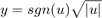
The subsystem implements three nonlinear functions, two of which are discontinuous. In combination, however, y is a continuous function of u.
Results
The model simulation uses the data loaded from the MAT file sldemo_hydcyl_data.mat. You can change parameter values via the Pump and Cylinder masks.


T = [0 0.04 0.04 0.05 0.05 0.1 ] sec
Q = [0.005 0.005 0 0 0.005 0.005] (m^3)/sec
Plot Simulation Results
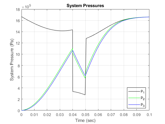
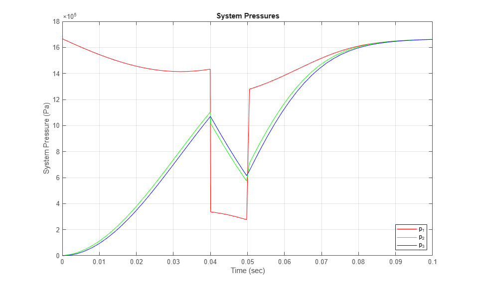
The system initially steps to a pump flow of 0.005 m^3/sec = 300 l/min, steps to zero at t=0.04 sec, and then resumes its initial flow rate at t=0.05 sec.
The control valve starts with zero orifice area and ramps to 1e-4 m^2 during the 0.1 sec simulation time. With the valve closed, all of the pump flow goes to leakage, so the initial pump pressure increases to p10 = Q/C2 = 1667 kPa.
As the valve opens, pressures p2 and p3 build up while p1 decreases in response to the load increase. When the pump flow cuts off, the spring and piston act like an accumulator, and p3 decreases continuously. Then, the flow reverses direction, so p2, though relatively close to p3, falls. At the pump itself, all of the back-flow leaks, and p1 drops. The behavior reverses as the flow is restored.
The piston position is directly proportional to p3, where the hydraulic and spring forces balance. Discontinuities in the velocity at 0.04 sec and 0.05 sec indicate negligible mass. The model reaches a steady state when all of the pump flow again goes to leakage, which is now due to a zero pressure-drop across the control valve when p3 = p2 = p1 = p10.
Plot the piston position, hidden code