Cumulative Coverage Analysis
This example illustrates the use of the Coverage Results Explorer to simplify the generation of cumulative coverage data and reports spanning a set of multiple coverage runs.
Open Example Model
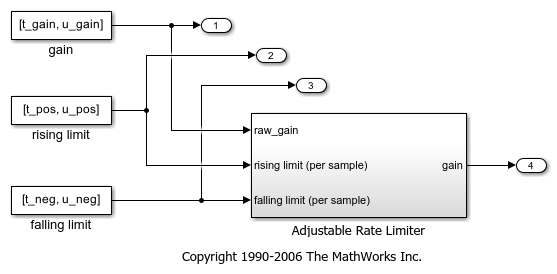
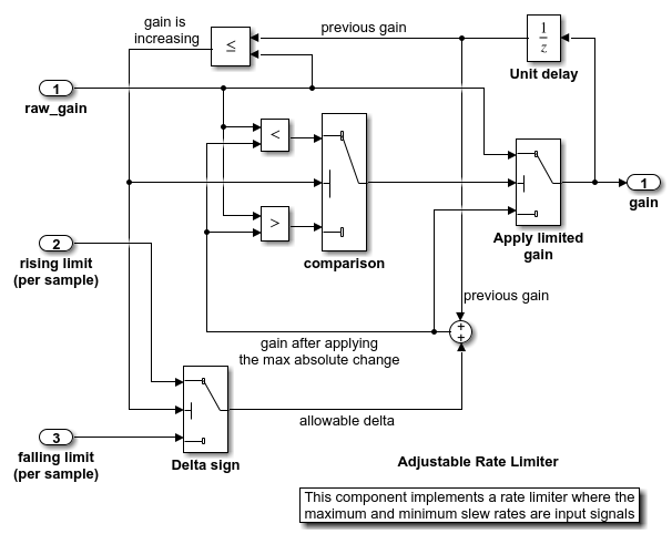
This example uses the slvnvdemo_ratelim_harness model to explain the settings and options to accumulate coverage. Inside this model is an implementation of an Adjustable Rate Limiter. It uses three Switch blocks to control when the output should be limited and the type of limit to apply.
Inputs are produced using three From Workspace blocks: gain, rising limit, and falling limit. The values of the inputs are specified by six variables defined in the MATLAB® workspace: t_gain, u_gain, t_pos, u_pos, t_neg, and u_neg.
open_system('slvnvdemo_ratelim_harness');
open_system('slvnvdemo_ratelim_harness/Adjustable Rate Limiter');
Enable Coverage Analysis
Start by opening the coverage settings. From the Modeling tab, select Model Settings.
To enable the coverage tool, select Enable coverage analysis in the Coverage pane. This setting enables the other options in the Coverage pane.
For this example, collect condition and decision coverage. Under the Coverage metrics panel, set the Structural coverage level to Condition Decision.
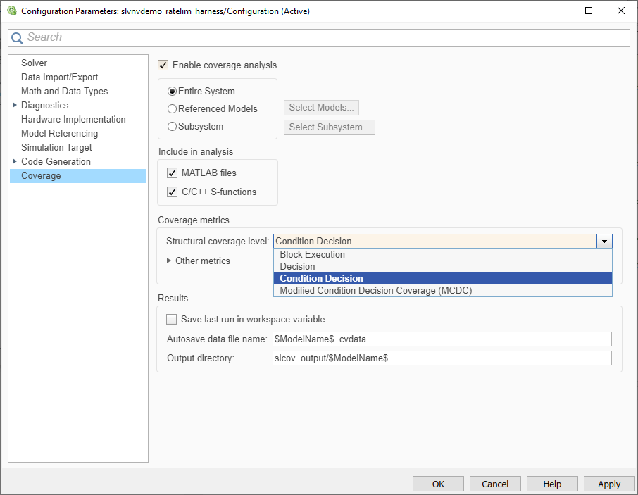
Click OK to apply your selected settings and close this dialog.
Simulate Model with First Test Case
The first test case exercises the scenario where the input values do not change rapidly. It uses a sine wave as the time varying signal and constants for rising and falling limits.
t_gain = (0:0.02:2.0)';
u_gain = sin(2*pi*t_gain);
Calculate the minimum and maximum change of the time varying input using the MATLAB diff function.
max_change = max(diff(u_gain))
min_change = min(diff(u_gain))
max_change =

    0.1253


min_change =

   -0.1253
Based on these minimum and maximum rates of change, set the rate limits to 1 and -1. As such, the rate of change of the input will be well within these limits for this test run.
t_pos = [0;2];
u_pos = [1;1];
t_neg = [0;2];
u_neg = [-1;-1];
Simulate the model with this first set of input variables by clicking the Run (Coverage) button.
Review First Test Case in Results Explorer
To open the Results Explorer, in the Coverage Analyzer app, click Results Explorer.
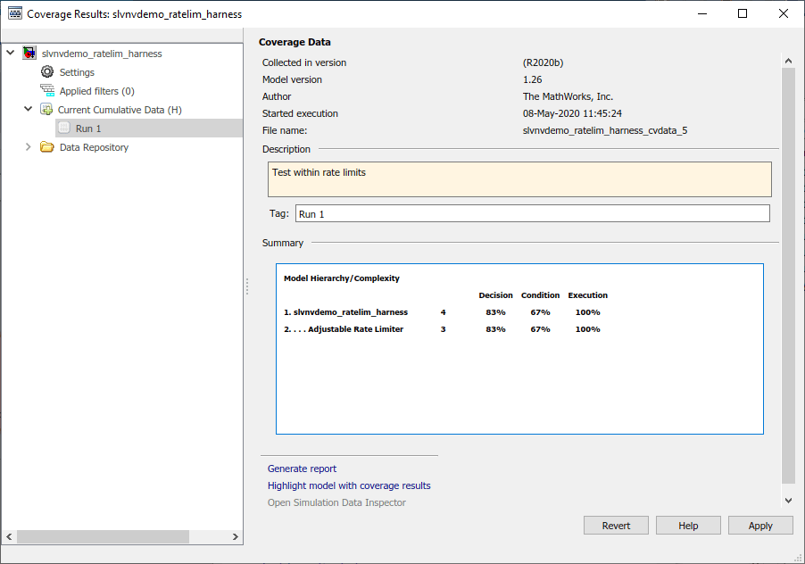
At this point the Current Cumulative Data contains just this first coverage run (tagged as Run 1). The Results Explorer initially shows information regarding this latest coverage run, including a summary of results for each enabled metric.
To keep track of the intent of this simulation, enter the text "Test within rate limits" in the Description field and click Apply.
Simulate Model with Second Test Case
The second test case complements the first case with a rising gain that exceeds the rate limit. After a second it increases the rate limit so that the gain changes are below that limit.
t_gain = [0;2];
u_gain = [0;4];
t_pos = [0;1;1;2];
u_pos = [1;1;5;5]*0.02;
t_neg = [0;2];
u_neg = [0;0];
Simulate the model with this second set of variables by clicking the Run (Coverage) button.
Generate Cumulative Progress Report for Second Test Case
Now that multiple coverage runs have been performed, you can generate cumulative coverage reports.
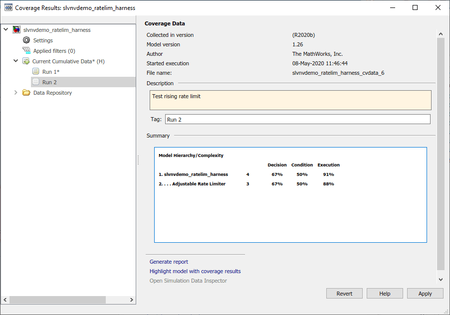
First, add a brief description of this run, as was done for the previous simulation. Enter the text "Test rising rate limit" in the Description field for Run 2 and click Apply.
There are different formats of coverage reports that can be generated. To visualize how the most recent simulation affects the cumulative coverage results, you can generate a cumulative progress report.
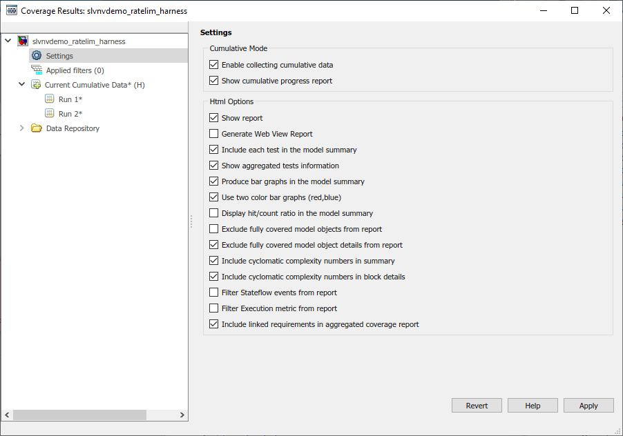
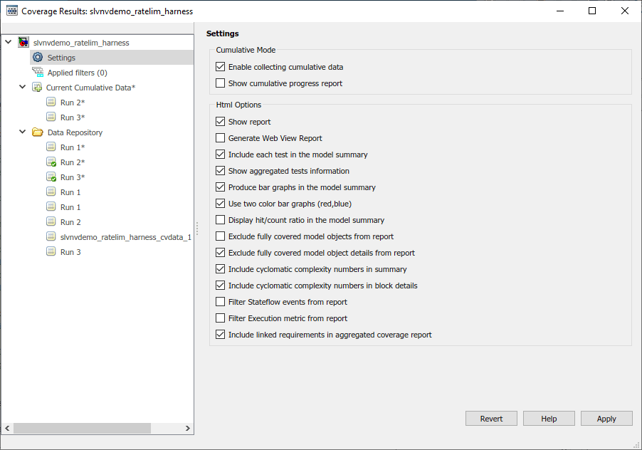
In the Results Explorer, under Settings, select Show cumulative progress report and click Apply.
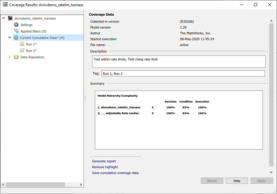
Click on Current Cumulative Data in the leftmost pane of the Results Explorer. Note that the Summary indicates the cumulative coverage results accumulated from Run 1 and Run 2. Click on Generate Report to create the cumulative progress report.
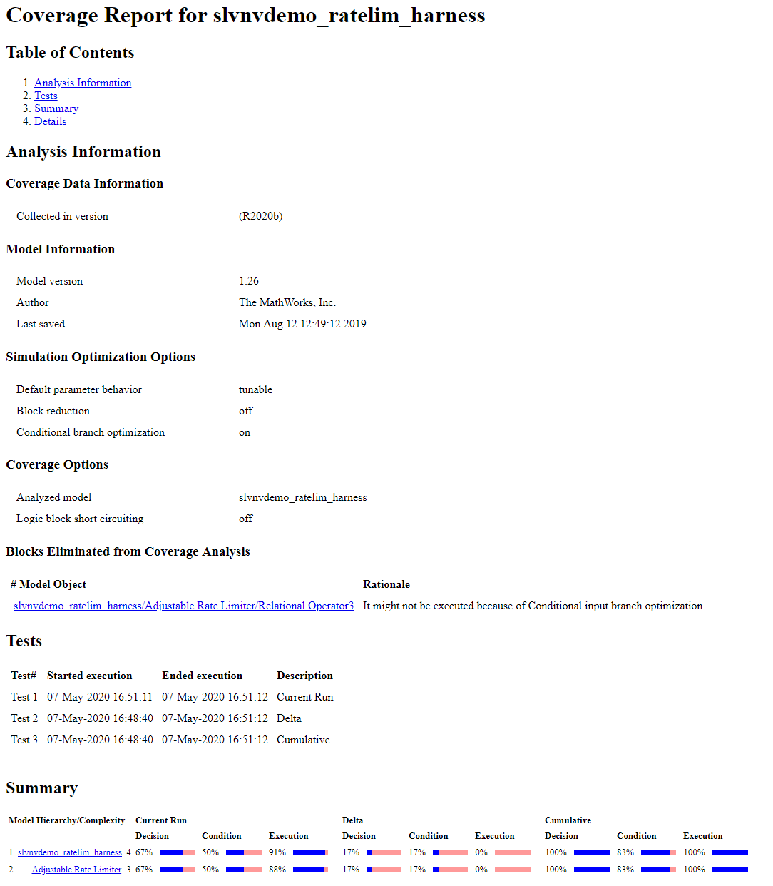
The Summary section of the cumulative progress report has three columns: Current Run, Delta, and Cumulative. The Current Run column displays the coverage from the last simulation listed under Current Cumulative Data (which is Run 2 in this case). The Delta column displays the coverage exposed by the current run that was not achieved in the cumulative results before this simulation. The Cumulative column gives the current cumulative coverage results.
Simulate Model with Third Test Case
The third test case is a mirror image of the second, with the rising gain replaced by a falling gain.
t_gain = [0;2];
u_gain = [-0.02;-4.02];
t_pos = [0;2];
u_pos = [0;0];
t_neg = [0;1;1;2];
u_neg = [-1;-1;-5;-5]*0.02;
Simulate the model with this third set of variables by clicking the Run (Coverage) button.
Generate Cumulative Progress Report for Third Test Case
Once again, add a brief description of the latest run. Enter the text "Test falling rate limit" in the Description field for Run 3 and click Apply.
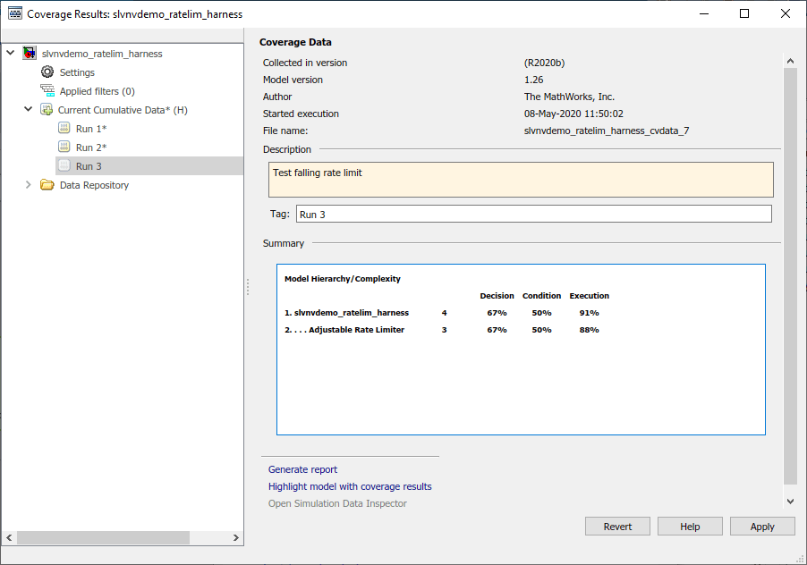
Navigate to Current Cumulative Data and click Generate Report to create a cumulative progress report for this latest run.
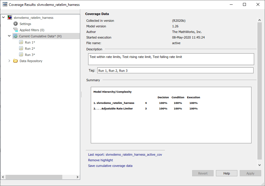
Notice that with this latest run, the cumulative results achieve full coverage for the Decision, Condition, and Execution metrics.
Refine Cumulative Dataset
If you determine that a particular coverage run is not necessary, you can exclude this run from the cumulative dataset and generate a new cumulative report.
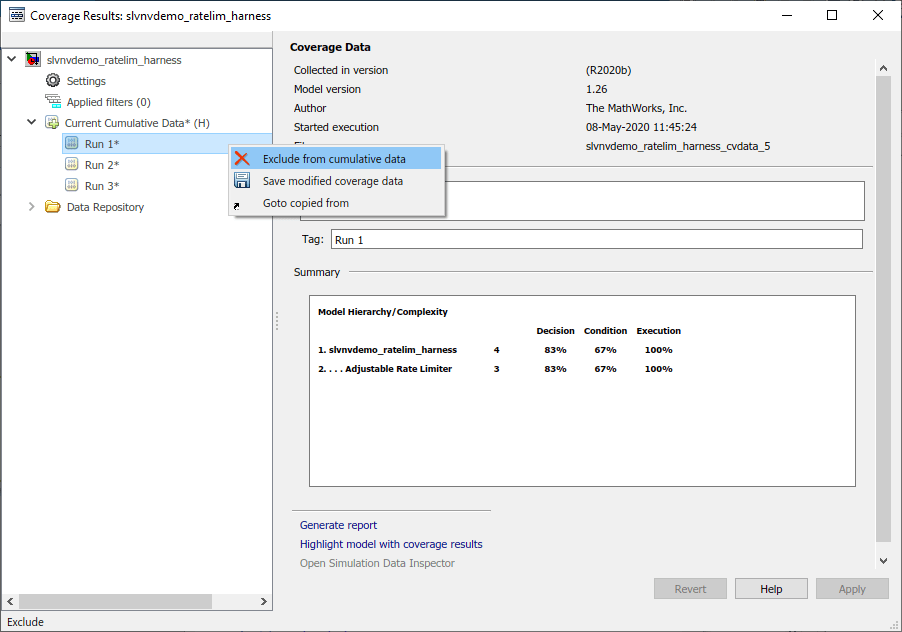
In the Results Explorer, under Current Cumulative Data, right-click on Run 1 and select Exclude from cumulative data.
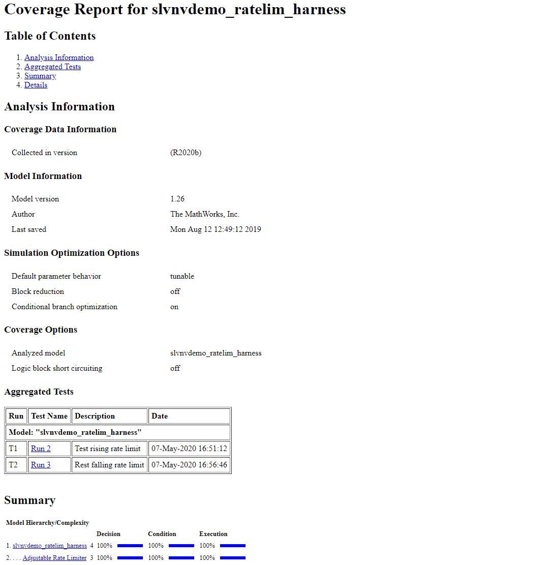
Generate Final Cumulative Coverage Report
Now that you have selected the desired subset of test runs, you can generate a coverage report for the accumulated results.
Navigate to Settings, deselect Show cumulative progress report, and then click Apply.
Navigate to Current Cumulative Data and click Generate Report.
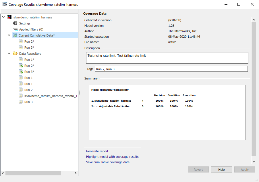
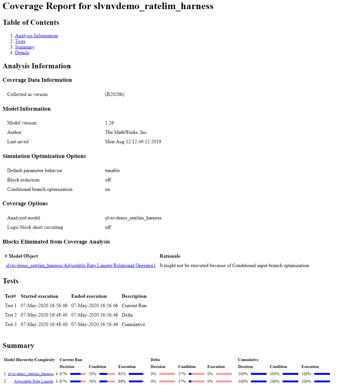
The cumulative coverage report displays the results associated with the current cumulative data. Notice under the Tests section, there is a single test with the description "Test rising rate limit,Test falling rate limit", indicating that this test contains the accumulated results from runs 2 and 3.
The Summary section shows that these cumulative results attain full coverage for all metrics analyzed.