Design Selection Using Multiobjective Tradeoff Analysis

Open Live Script

This example shows how to select designs by performing a multiobjective tradeoff analysis using the Sensitivity Analyzer app. You explore the design of a continuously stirred tank reactor (CSTR) to minimize product concentration variation and production cost.

You explore the CSTR design by sampling the design variables and evaluating the design for each combination of design variables. You then create a multiobjective scatter plot to visualize optimal designs in the objective space, select the design that best satisfies the tradeoff between the design objectives, and analyze feasibility trends in the generated designs.

Continuously Stirred Tank Reactor (CSTR) Model

Continuously stirred tank reactors (CSTRs) are common in the process industry. The Simulink® model, sdoCSTR, models a jacketed diabatic, that is, non-adiabatic tank reactor described in [1]. The CSTR is assumed to be perfectly mixed, with a single first-order exothermic and irreversible reaction, $A \to B$ . $A$ , the reactant, is converted to $B$ , the product.

In this example, you use the following two-state CSTR model, which uses basic accounting and energy conservation principles:

$\frac{d C_{A}}{d t} = \frac{F}{A \cdot h} (C_{f e e d} - C_{A}) - r \cdot C_{A}$

$\frac{d T}{d t} = \frac{F}{A \cdot h} (T_{f e e d} - T) - \frac{H}{c_{p} \cdot ρ} r - \frac{U}{c_{p} \cdot ρ \cdot h} (T - T_{c o o l})$

$r = k_{0} \cdot e^{\frac{- E}{R \cdot T}}$

$C_{A}$ and $C_{f e e d}$ — Concentrations of $A$ in the CSTR and in the feed respectively [ $k g m o l / m^{3}$ ]
$T$ , $T_{f e e d}$ , and $T_{c o o l}$ — CSTR, feed, and coolant temperatures respectively [ $K$ ]
$F$ — Volumetric flow rate in the CSTR [ $m^{3} / h$ ]
$ρ$ — Density of the material in the CSTR [ $1 / m^{3}$ ]
$h$ — Height of the CSTR [ $m$ ]
$A$ — Heated cross-sectional area of the CSTR [ $m^{2}$ ]
$k_{0}$ — Pre-exponential non-thermal factor for reaction [ $1 / h$ ]
$E$ and $H$ — Activation energy and heat of reaction respectively [ $k c a l / k g m o l$ ]
$R$ — Boltzmann's gas constant [ $k c a l / (k g m o l \cdot K)$ ]
$c_{p}$ — Heat capacity coeffiecient [ $k c a l / K$ ]
$U$ — Heat transfer coefficient [ $k c a l / (m^{2} \cdot K \cdot h)$ ]

Open the Simulink model.

open_system('sdoCSTR');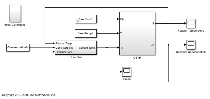

Design Problem

Assume that the CSTR is cylindrical, with the coolant applied to the base of the cylinder. The variables available for tuning the design are:

The CSTR design variables — CSTR cross-sectional area (A) and height (h).
The feed variables — feed concentration (FeedCon0) and temperature (FeedTemp0).

The design goals are:

To minimize the variation in residual concentration, $C_{A}$ , as these variations negatively affect the quality of the CSTR product. Minimizing the variations also improves CSTR profit.
To minimize the mean coolant temperature, $T_{c o o l}$ , as heating or cooling the jacket coolant is expensive. Minimizing the mean coolant temperature improves CSTR profit.
To maintain the CSTR temperature, $T$ , below $353 K (8 0^{\circ} C)$ for safety purposes.

Specify Design Variables and Create the Design Space

To open the Sensitivity Analyzer app, in the Simulink model window, in the Apps gallery, click Sensitivity Analyzer.

To create a new parameter set, in the Sensitivity Analysis tab, in the Select Parameters drop-down list, select New. In the Select Parameters dialog box, select the CSTR design variables A and h and the feed variables FeedCon0 and FeedTemp0. Click OK.

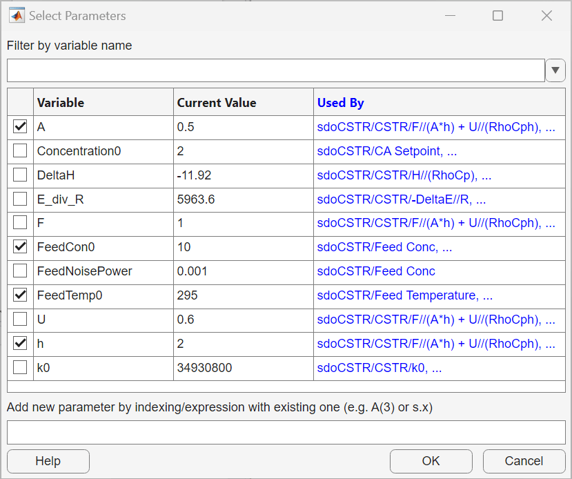
A new ParamSet appears in the Parameter Sets section of the app which contains the selected parameters.

To create a gridded space of parameter values, select ParamSet and in the Sensitivity Analysis tab, in the Generate Values drop-down list, select Generate Gridded Values. In the Generate Gridded Parameter Values dialog box, specify the Starting Values of the selected parameters as ranging from:

$1.5 m^{2}$ to $2.5 m^{2}$ in increments of $0.5 m^{2}$ for A
$5 k g m o l / m^{3}$ to $15 k g m o l / m^{3}$ in increments of $5 k g m o l / m^{3}$ for FeedCon0
$290 K$ to $320 K$ in increments of $10 K$ for FeedTemp0
$1.5 m$ to $3 m$ in increments of $0.5 m$ for h

To create an exhaustive combination of parameter values, select All Combinations as the Gridding Method and click OK.

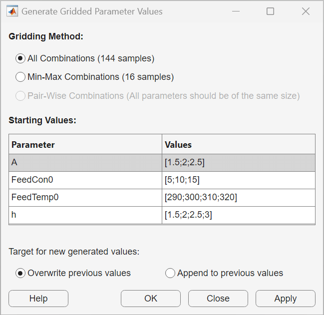
Doing so populates the parameter set paramSet with the parameter combinations.

Specify Objectives and Constraints for Evaluation

Specify the requirements that serve as the objectives and constraints for the design problem, based on the design goals.

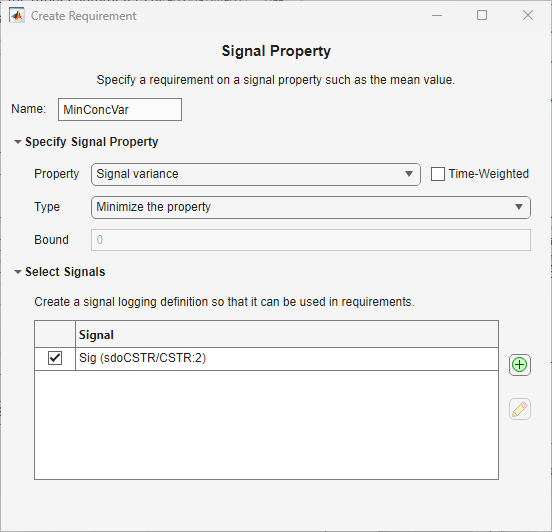
To specify the objective to minimize the residual concentration variation, in the Sensitivity Analysis tab, in the New Requirement drop-down list, select Signal Property. In the Create Requirement dialog box:

In the Specify Signal Property area, in the Property drop-down list, select Signal variance, and in the Type drop-down list, select Minimize the property.
In the Select Signals area, click the add button and select the signal at the output, CA, of the CSTR block. In the Create Signal Set dialog box, click OK.

Close the Create Requirement dialog box. A new requirement SignalProperty appears in the Requirements section of the app. Rename the requirement as MinConcVar by slowly double-clicking on it. To open the Create Requirement dialog box for this requirement again, right-click on MinConcVar and click Edit.

To specify the objective to minimize the mean coolant temperature, in the Sensitivity Analysis tab, in the New Requirement drop-down list, select Signal Property. In the Create Requirement dialog box:

In the Specify Signal Property area, in the Property drop-down list, select Signal mean, and in the Type drop-down list, select Minimize the property.
In the Select Signals area, click the add button and select the signal at the output, Coolant Temp., of the Controller block. In the Create Signal Set dialog box, click OK.

Close the Create Requirement dialog box. Rename the requirement SignalProperty as MinCoolTemp.

To specify an upper bound constraint on the CSTR temperature, in the Sensitivity Analysis tab, in the New Requirement drop-down list, select Signal Bound. In the Create Requirement dialog box:

In the Specify Signal Bound area, in the Type drop-down list, select Constrain signal to be <= the bound. Enter Start Time as 0 and End Time as 60. Enter Start Amplitude and End Amplitude as 353.
In the Select Signals to Bound area, click the add button and select the signal at the output, T, of the CSTR block. In the Create Signal Set dialog box, click OK.

Close the Create Requirement dialog box. Rename the requirement SignalBound as ReacTempUB.

Evaluate the Designs and Plot the Multiobjective Objective Space

In the Sensitivity Analysis tab, click Select for Evaluation. In the Select for Evaluation dialog box, you can see that all requirements are selected to be evaluated by default. Click Close.

To evaluate the MinConcVar, MinCoolTemp, and ReacTempUB requirements for each row of parameter values in ParamSet, in the Sensitivity Analysis tab, click Evaluate Model.

To speed up evaluation, you can:

Disable the default scatter plot update setting to update the plots only after all evaluations are complete. To do this, in the Sensitivity Analysis tab, in the dropdown list for Options, click General. In the Evaluation Options dialog box, under the General tab, uncheck Update scatter plots during evaluation and click OK.
Use parallel computing if you have Parallel Computing Toolbox™. For more information, see Use Parallel Computing for Sensitivity Analysis.
Use fast restart. For more information, see Use Fast Restart Mode During Sensitivity Analysis.

The results appear as a new evaluation result EvalResult in the Results section of the app. Rename the result as AllOutcomes.

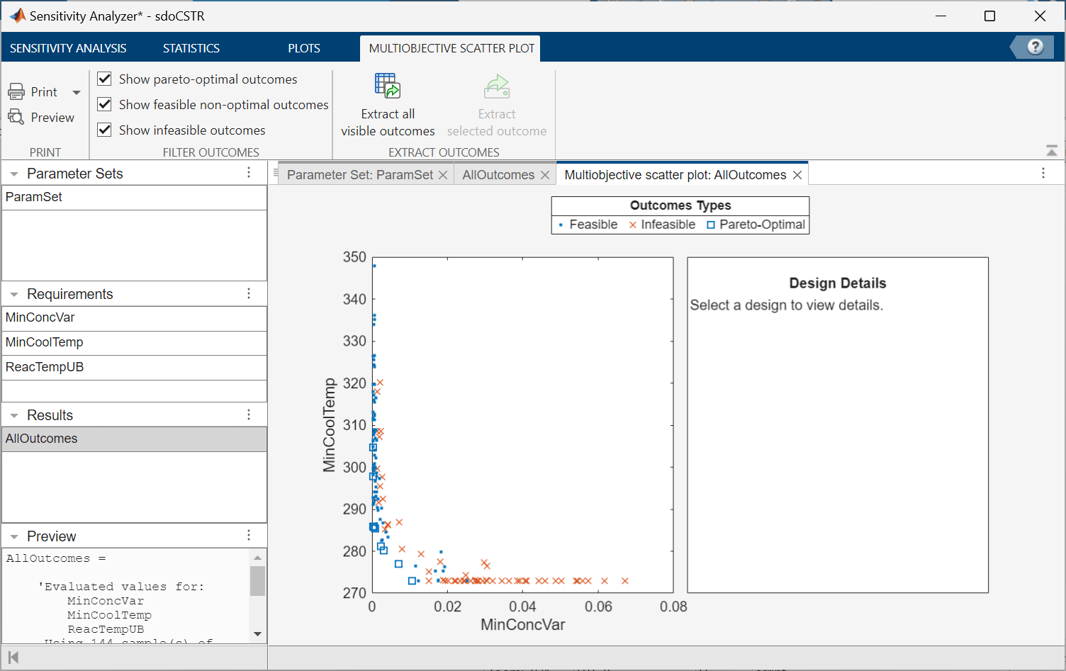
You can create a multiobjective scatter plot for any evaluation result containing two or more objectives. Select AllOutcomes and in the Plots tab, click Multiobjective scatter plot.

Analyze the Pareto-Optimal Designs

By default, the multiobjective scatter plot shows the objective values for all possible combinations of the parameters. To view only the pareto-optimal designs, in the Multiobjective Scatter Plot tab, uncheck the Show feasible non-optimal outcomes and Show infeasible outcomes options.

The filtered view of the multiobjective scatter plot shows the tradeoff between minimizing the concentration variation and minimizing the mean coolant temperature. As the concentration variation of the optimal outcomes decreases, the mean coolant temperature tends to increase. After decreasing the concentration variation to approximately $3.17 \times 1 0^{- 5}$ , further decreasing the concentration variation results in a substantial increase in the coolant temperature. This design outcome, or "knee point", provides an optimal tradeoff between minimizing concentration variation and mean coolant temperature.

Select the "knee point" design to view its design details. To export the parameter values at this design outcome, in the Multiobjective Scatter Plot tab, click Extract selected outcome. A new parameter set ParamValues appears in the Results section of the app. Rename ParamValues as SelectedDesign.

Analyze the Infeasible Designs

To view only the infeasible designs, in the Multiobjective Scatter Plot tab, check only the Show infeasible outcomes option.

To export data corresponding to the infeasible outcomes, in the Multiobjective Scatter Plot tab, click Extract all visible outcomes. The infeasible outcomes data appears as a new evaluation result EvalResult in the Results section of the app. Rename the evaluation result as InfeasibleOutcomes.

To analyze the parameters-requirements distributions for the infeasible designs, select InfeasibleOutcomes and in the Plots tab, click Scatter plot. From the scatter plot, you can observe that:

A design using a higher initial feed concentration (FeedConc0) mostly ends up with an infeasible design. None of the infeasible designs result from an initial feed concentration of $5 k g m o l / m^{3}$ .
Most of the infeasible designs occur when trying to achieve a mean coolant temperature below $280 K$ .

To directly view and analyze the results obtained in this example, open the session sdoCSTR_sasession.mat.

Close the model.

bdclose('sdoCSTR');

References

[1] Bequette, B.W. Process Dynamics: Modeling, Analysis and Simulation. 1st ed. Upper Saddle River, NJ: Prentice Hall, 1998.