Identify Key Parameters for Estimation (Code)
This example shows how to use sensitivity analysis to narrow down the number of parameters that you need to estimate to fit a model. This example uses a model of the vestibulo-ocular reflex, which generates compensatory eye movements.
Model Description
The vestibulo-ocular reflex (VOR) enables the eyes to move at the same speed and in the opposite direction as the head, so that vision is not blurred when the head moves during normal activity. For example, if the head turns in one direction, the eyes turn in the opposite direction, with the same speed. This happens even in the dark. In fact, the VOR is most easily characterized by measurements in the dark, to ensure that eye movements are predominantly driven by the VOR.
The file sdoVOR_Data.mat contains uniformly sampled data of stimulation and eye movements. If the VOR were perfectly compensatory, then a plot of eye movement data, when flipped vertically, would overlay exactly on top of a plot of head motion data. Such a system would be described by a gain of 1 and a phase of 180 degrees. However, when we plot the data in the file sdoVOR_Data.mat, the eye movements are close, but not perfectly compensatory.
load sdoVOR_Data.mat;   % Column vectors:   Time  HeadData  EyeData
figure
plot(Time, HeadData, ':b',    Time, EyeData, '-g')
xlabel('Time (sec)')
ylabel('Angular  Velocity  (deg/sec)')
ylim([-110  110])
legend('Head Data', 'Eye Data')
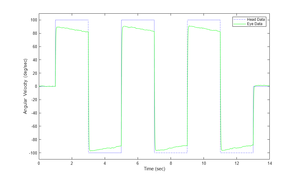
The eye movement data does not perfectly overlay the head motion data, and this can be modeled by several factors. Head rotation is sensed by organs in the inner ears, known as semicircular canals. These detect head motion and transmit signals about head motion to the brain, which sends motor commands to the eye muscles, so that eye movements compensate for head motion. We would like to use this eye movement data to estimate the parameters in the models for these various stages. The model we will use is shown below. There are four parameters in the model: Delay, Gain, Tc, and Tp.
model_name = 'sdoVOR';
open_system(model_name)
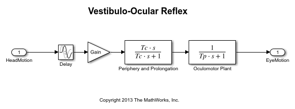
The Delay parameter models the fact that there is some delay in communicating the signals from the inner ear to the brain and the eyes. This delay is due to the time needed for chemical neurotransmitters to traverse the synaptic clefts between nerve cells. Based on the number of synapses involved in the vestibulo-ocular reflex, this delay is expected to be around 5 ms. For estimation purposes, we will assume it is between 2 and 9 ms.
Delay = sdo.getParameterFromModel(model_name, 'Delay');
Delay.Value = 0.005;   % seconds
Delay.Minimum = 0.002;
Delay.Maximum = 0.009;
The Gain parameter models the fact that the eyes do not move quite as much as the head does. We will use 0.8 as our initial guess, and assume it is between 0.6 and 1.
Gain = sdo.getParameterFromModel(model_name, 'Gain');
Gain.Value = 0.8;
Gain.Minimum = 0.6;
Gain.Maximum = 1;
The Tc parameter models the dynamics associated with the semicircular canals, as well as some additional neural processing. The canals are high-pass filters, because after a subject has been put into rotational motion, the neurally active membranes in the canals slowly relax back to resting position, so the canals stop sensing motion. Thus in the plot above, after the stimulation undergoes transition edges, the eye movements tend to depart from the stimulation over time. Based on mechanical characteristics of the canals, combined with additional neural processing which prolongs this time constant to improve the accuracy of the VOR, we will estimate the Tc parameter to be 15 seconds, and assume it is between 10 and 30 seconds.
Tc = sdo.getParameterFromModel(model_name, 'Tc');
Tc.Value = 15;
Tc.Minimum = 10;
Tc.Maximum = 30;
Finally, the Tp parameter models the dynamics of the oculomotor plant, i.e. the eye and the muscles and tissues attached to it. The plant can be modeled by two poles, however it is believed that the pole with the larger time constant is canceled by precompensation in the brain, to enable the eye to make quick movements. Thus in the plot, when the stimulation undergoes transition edges, the eye movements follow with only a little delay. For the Tp parameter, we will use 0.01 seconds as our initial guess, and assume it is between 0.005 and 0.05 seconds.
Tp = sdo.getParameterFromModel(model_name, 'Tp');
Tp.Value = 0.01;
Tp.Minimum = 0.005;
Tp.Maximum = 0.05;
Collect these parameters into a vector.
v = [Delay Gain Tc Tp];
Compare Measured Data to Initial Simulated Output
Create an Experiment object. Specify HeadData as input.
Exp = sdo.Experiment(model_name);
Exp.InputData = timeseries(HeadData, Time);
Associate eye movement data with model output.
EyeMotion = Simulink.SimulationData.Signal;
EyeMotion.Name = 'EyeMotion';
EyeMotion.BlockPath = [model_name  '/Oculomotor Plant'];
EyeMotion.PortType = 'outport';
EyeMotion.PortIndex = 1;
EyeMotion.Values = timeseries(EyeData, Time);
Add EyeMotion to the experiment.
Exp.OutputData = EyeMotion;
Use the data's timing characteristics in the model.
stop_time = Time(end);
set_param(gcs, 'StopTime', num2str(stop_time));
dt = Time(2) - Time(1);
set_param(gcs, 'FixedStep', num2str(dt))
Create a simulation scenario using the experiment, and obtain the simulated output.
Exp = setEstimatedValues(Exp, v);   % use vector of parameters/states
Simulator = createSimulator(Exp);
Simulator = sim(Simulator);
Search for the model_residual signal in the logged simulation data.
SimLog = find(Simulator.LoggedData,  ...
	get_param(model_name, 'SignalLoggingName') );
EyeSignal = find(SimLog, 'EyeMotion');
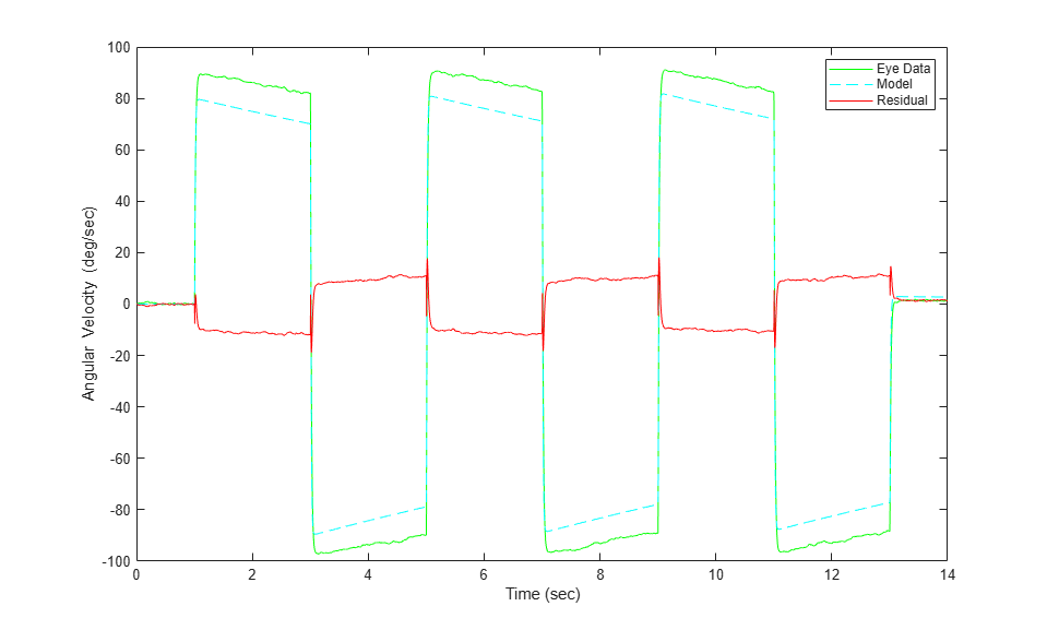
The model output does not match the data very well, as shown by the residual, which we can compute by calling the objective function.
estFcn = @(v) sdoVOR_Objective(v, Simulator, Exp, 'Residuals');
Model_Error = estFcn(v);
plot(Time, EyeData, '-g',  ...
	EyeSignal.Values.Time, EyeSignal.Values.Data, '--c',  ...
	Time, Model_Error.F, '-r');
xlabel('Time (sec)');
ylabel('Angular  Velocity  (deg/sec)');
legend('Eye Data', 'Model', 'Residual');
The objective function used above is defined in the file "sdoVOR_Objective.m".
type sdoVOR_Objective.m
function vals = sdoVOR_Objective(v, Simulator, Exp, Method)
% Compare model output with data
%
%    Inputs:
%       v - vector of parameters and/or states
%       Simulator - used to simulate the model
%       Exp - Experiment object
%       Method - 'SSE' for scalar output, 'Residuals' for vector of residuals

% Copyright 2014-2015 The MathWorks, Inc.

% Requirement setup
req = sdo.requirements.SignalTracking;
req.Type = '==';
req.Method = Method;

% If Residuals requested, keep on same scale as signals, for plotting
switch Method
	case 'Residuals'
		req.Normalize = 'off';
end

% Simulate the model
Exp = setEstimatedValues(Exp, v);   % use vector of parameters/states
Simulator = createSimulator(Exp,Simulator);
Simulator = sim(Simulator);

% Compare model output with data
SimLog = find(Simulator.LoggedData,  ...
	get_param(Exp.ModelName, 'SignalLoggingName') );
OutputModel = find(SimLog, 'EyeMotion');
Model_Error = evalRequirement(req, OutputModel.Values, Exp.OutputData.Values);
vals.F = Model_Error;
Sensitivity Analysis
Create an object to sample the parameter space.
ps = sdo.ParameterSpace([Delay ; Gain ; Tc ; Tp]);
Generate 100 samples from the parameter space.
rng default;   % for reproducibility
x  = sdo.sample(ps, 100);
sdo.scatterPlot(x);
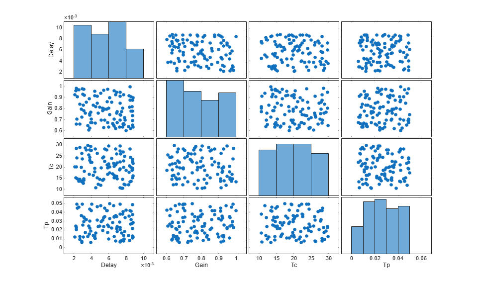
The sampling above used default options, and these are reflected in the plots above. Parameter values were selected at random from distributions that were uniform over the range of each parameter. Consequently, the histogram plots along the diagonal appear approximately uniform. If Statistics and Machine Learning Toolbox™ is available, many other distributions may be used, and sampling can be done using Sobol or Halton low-discrepancy sequences.
The off-diagonal plots above show scatter plots between pairs of different variables. Since we did not specify a RankCorrelation matrix in ps, the scatter plots do not indicate correlations. However, if parameters were believed to be correlated, this can be specified using the RankCorrelation property of ps.
For sensitivity analysis, it is simpler to use a scalar objective, so we will specify the sum of squared errors, "SSE":
estFcn = @(v) sdoVOR_Objective(v, Simulator, Exp, 'SSE');
y = sdo.evaluate(estFcn, ps, x);
Model evaluated at 100 samples.
Evaluation could also be sped up using parallel computing.
Obtain the standardized regression coefficients.
opts = sdo.AnalyzeOptions;
opts.Method = 'StandardizedRegression';
sensitivities = sdo.analyze(x, y, opts);
Other types of analysis include correlation and, if Statistics and Machine Learning Toolbox is available, partial correlation.
We can view the analysis results.
disp(sensitivities)
                 F
             _________

    Delay      0.01303
    Gain      -0.90873
    Tc       -0.044395
    Tp         0.19919
For standardized regression, parameters that highly influence the model output have sensitivity magnitudes close to 1. On the other hand, less influential parameters have smaller sensitivity magnitudes. We see that this objective function is sensitive to changes in the Gain and Tp parameters, but much less sensitive to changes in the Delay and Tc parameters.
You can validate sensitivity analysis results by resampling and reevaluating the objective function for the samples. You can also use engineering intuition for a quick analysis. For example, in this model, the time constant Tc ranges from 10 to 30 seconds. Even the minimum value of 10 seconds is large compared to the 2-second duration for which the head motion stimulation is held at constant velocity. Therefore, Tc is not expected to affect the output greatly. However, even when this kind of intuition is not readily available in other models, sensitivity analysis can help highlight which parameters are influential.
Based on the results of sensitivity analysis, designate the Delay and Tc parameters as fixed when optimizing. This reduction in the number of free parameters speeds up optimization.
Delay.Free = false;
Tc.Free = false;
Optimization
We can use the minimum from sensitivity analysis as the initial guess for optimization.
[fval, idx_min] = min(y.F);
Delay.Value = x.Delay(idx_min);
Gain.Value = x.Gain(idx_min);
Tc.Value = x.Tc(idx_min);
Tp.Value = x.Tp(idx_min);
%
v = [Delay Gain Tc Tp];
opts = sdo.OptimizeOptions;
opts.Method = 'fmincon';
As was the case with model evaluations in sensitivity analysis, parallel computing could be used to speed up the optimization.
vOpt = sdo.optimize(estFcn, v, opts);
disp(vOpt)
 Optimization started 2026-Apr-19, 07:00:12

                               max                     First-order
 Iter F-count        f(x)   constraint    Step-size    optimality
    0      5      13.4798            0
    1     18      12.2052            0        0.129          305
    2     30      11.1441            0       0.0648          790
    3     41      10.0493            0       0.0843          290
    4     46      9.23607            0       0.0758          286
    5     51      8.76122            0       0.0183         10.1
    6     56      8.75862            0      0.00184        0.476
    7     57      8.75862            0     8.41e-05        0.476
Local minimum possible. Constraints satisfied.

fmincon stopped because the size of the current step is less than
the value of the step size tolerance and constraints are
satisfied to within the value of the constraint tolerance.

(1,1) =

       Name: 'Delay'
      Value: 0.0038
    Minimum: 0.0020
    Maximum: 0.0090
       Free: 0
      Scale: 0.0078
       Info: [1×1 struct]


(1,2) =

       Name: 'Gain'
      Value: 0.9012
    Minimum: 0.6000
    Maximum: 1
       Free: 1
      Scale: 1
       Info: [1×1 struct]


(1,3) =

       Name: 'Tc'
      Value: 16.6833
    Minimum: 10
    Maximum: 30
       Free: 0
      Scale: 16
       Info: [1×1 struct]


(1,4) =

       Name: 'Tp'
      Value: 0.0157
    Minimum: 0.0050
    Maximum: 0.0500
       Free: 1
      Scale: 0.0156
       Info: [1×1 struct]


1x4 param.Continuous
Visualizing Result of Optimization
Obtain the model response after estimation. Search for the model_residual signal in the logged simulation data.
Exp = setEstimatedValues(Exp, vOpt);
Simulator = createSimulator(Exp,Simulator);
Simulator = sim(Simulator);
SimLog = find(Simulator.LoggedData,  ...
	get_param(model_name, 'SignalLoggingName') );
EyeSignal = find(SimLog, 'EyeMotion');
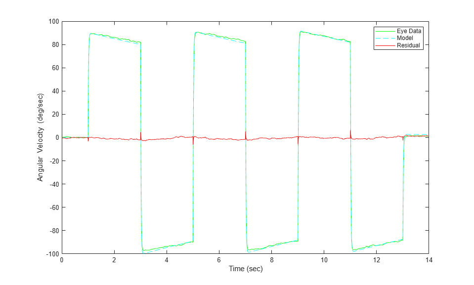
Comparing the measured eye data with the optimized model response shows that the residuals are much smaller.
estFcn = @(v) sdoVOR_Objective(v, Simulator, Exp, 'Residuals');
Model_Error = estFcn(vOpt);
plot(Time, EyeData, '-g',  ...
	EyeSignal.Values.Time, EyeSignal.Values.Data, '--c',  ...
	Time, Model_Error.F, '-r');
xlabel('Time (sec)');
ylabel('Angular  Velocity  (deg/sec)');
legend('Eye Data', 'Model', 'Residual');
Close the model.
bdclose(model_name)