Fit a Nonparametric Distribution with Pareto Tails
This example shows how to fit a nonparametric probability distribution to sample data using Pareto tails to smooth the distribution in the tails.
Step 1. Generate sample data.
Generate sample data that contains more outliers than expected from a standard normal distribution.
rng('default')  % For reproducibility
left_tail = -exprnd(1,10,1);
right_tail = exprnd(5,10,1);
center = randn(80,1);
data = [left_tail;center;right_tail];
The data contains 80% values from a standard normal distribution, 10% from an exponential distribution with a mean of 5, and 10% from an exponential distribution with mean of -1. Compared to a standard normal distribution, the exponential values are more likely to be outliers, especially in the upper tail.
Step 2. Fit probability distributions to the data.
Fit a normal distribution and a t location-scale distribution to the data, and plot for a visual comparison.
probplot(data);
hold on
p = fitdist(data,'tlocationscale');
h = plot(gca,p,'PlotType',"probability");
set(h,'color','r','linestyle','-');
title('Probability Plot')
legend('Normal','Data','t location-scale','Location','SE')
hold off
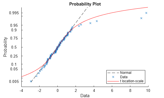
Both distributions appear to fit reasonably well in the center, but neither the normal distribution nor the t location-scale distribution fit the tails very well.
Step 3. Generate an empirical distribution.
To obtain a better fit, use ecdf to generate an empirical cdf based on the sample data.
figure
ecdf(data)
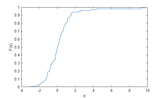
The empirical distribution provides a perfect fit, but the outliers make the tails very discrete. Random samples generated from this distribution using the inversion method might include, for example, values near 4.33 and 9.25, but no values in between.
Step 4. Fit a distribution using Pareto tails.
Use paretotails to generate an empirical cdf for the middle 80% of the data and fit generalized Pareto distributions to the lower and upper 10%.
pfit = paretotails(data,0.1,0.9)
pfit =
Piecewise distribution with 3 segments
      -Inf < x < -1.24623    (0 < p < 0.1): lower tail, GPD(-0.334156,0.798745)
   -1.24623 < x < 1.48551  (0.1 < p < 0.9): interpolated empirical cdf
        1.48551 < x < Inf    (0.9 < p < 1): upper tail, GPD(1.23681,0.581868)
To obtain a better fit, paretotails fits a distribution by piecing together an ecdf or kernel distribution in the center of the sample, and smooth generalized Pareto distributions (GPDs) in the tails. Use paretotails to create paretotails probability distribution object. You can access information about the fit and perform further calculations on the object using the object functions of the paretotails object. For example, you can evaluate the cdf or generate random numbers from the distribution.
Step 5. Compute and plot the cdf.
Compute and plot the cdf of the fitted paretotails distribution.
x = -4:0.01:10;
plot(x,cdf(pfit,x))
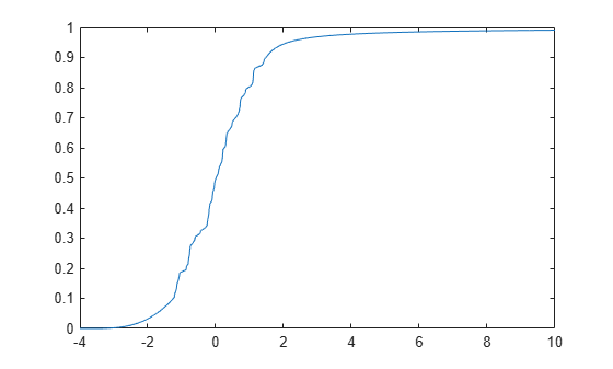
The paretotails cdf closely fits the data but is smoother in the tails than the ecdf generated in Step 3.
See Also
fitdist | paretotails | ecdf