Contenu principal

johnsrnd

Johnson system random numbers

Description

r = johnsrnd(quantiles) generates a random number drawn from the distribution in the Johnson system that satisfies the quantile specification given by quantiles.

r = johnsrnd(quantiles,sz1,...,szN) generates an array of random numbers, where sz1,...,szN indicates the size of each dimension.

example

r = johnsrnd(quantiles,sz) generates an array of random numbers, where the vector sz specifies size(r).

[r,type] = johnsrnd(___) also returns the type of the specified distribution within the Johnson system, using any of the input argument combinations in the previous syntaxes. To identify the distribution type without generating any random numbers, specify [r,type] = johnsrnd(quantiles,0).

[r,type,coefs] = johnsrnd(___) also returns the coefficients coefs of the transformation corresponding to the specified Johnson distribution type.

Examples

collapse all

Generate random numbers using different Johnson system distributions.

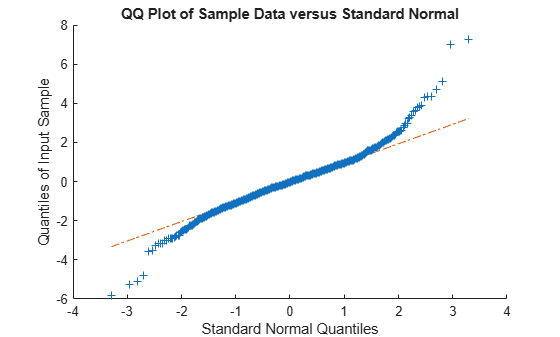
Generate random numbers with longer tails than a standard normal distribution.

rng default;  % For reproducibility
r = johnsrnd([-1.7 -.5 .5 1.7],1000,1);
figure;
qqplot(r);

Figure contains an axes object. The axes object with title QQ Plot of Sample Data versus Standard Normal, xlabel Standard Normal Quantiles, ylabel Quantiles of Input Sample contains 3 objects of type line. One or more of the lines displays its values using only markers

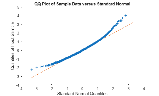
Generate random numbers skewed to the right.

r = johnsrnd([-1.3 -.5 .5 1.7],1000,1);
figure;
qqplot(r);

Figure contains an axes object. The axes object with title QQ Plot of Sample Data versus Standard Normal, xlabel Standard Normal Quantiles, ylabel Quantiles of Input Sample contains 3 objects of type line. One or more of the lines displays its values using only markers

Generate random numbers that match sample data well in the right tail.

load carbig;
qnorm = [.5 1 1.5 2];
q = quantile(Acceleration, normcdf(qnorm));
r = johnsrnd([qnorm;q],1000,1);
[q;quantile(r,normcdf(qnorm))]
ans = 2×4

   16.7000   18.2086   19.5376   21.7263
   16.6986   18.2220   19.9078   22.0918

Determine the distribution type and the coefficients.

[r,type,coefs] = johnsrnd([qnorm;q],0)
r =

     []
type = 
'SU'
coefs = 1×4

    1.0920    0.5829   18.4382    1.4494

Input Arguments

collapse all

Quantiles of the Johnson distribution type, specified as a four-element numeric vector of monotonically increasing values, or as a 2-by-4 numeric matrix. The elements of quantiles are the quantiles for the intended distribution that correspond to the standard normal quantiles [–1.5 –0.5 0.5 1.5]. In other words, you specify a distribution from which to draw random numbers by designating quantiles that correspond to the cumulative probabilities [0.067 0.309 0.691 0.933].

When quantiles is a 2-by-4 matrix, the first row contains four standard normal quantiles, and the second row contains the corresponding quantiles of the intended distribution. The standard normal quantiles must be spaced evenly.

Data Types: single | double

Size of each dimension, specified as separate arguments of integers. For example, specifying 5,3,2 generates a 5-by-3-by-2 array of random numbers from the probability distribution.

  • If you specify a single value sz1, then r is a square matrix of size sz1-by-sz1.

  • If the size of any dimension is 0 or negative, then r is an empty array.

  • Beyond the second dimension, johnsrnd ignores trailing dimensions with a size of 1. For example, specifying 1,4,1,1,1,1 produces a 1-by-4 vector of random numbers.

Data Types: single | double

Size of each dimension, specified as a row vector of integers. For example, specifying [5,3,2] generates a 5-by-3-by-2 array of random numbers from the probability distribution.

  • If you specify a single value [sz1], then r is a square matrix of size sz1-by-sz1.

  • If the size of any dimension is 0 or negative, then r is an empty array.

  • Beyond the second dimension, johnsrnd ignores trailing dimensions with a size of 1. For example, specifying [1,4,1,1,1,1] produces a 1-by-4 vector of random numbers.

Data Types: single | double

Output Arguments

collapse all

Johnson system random numbers, returned as a scalar value or an array of scalar values with the dimensions specified by sz1,...,szN or sz. Each element in r is a random number generated from the distribution specified by the quantiles in quantiles.

Type of Johnson distribution, returned as a character vector containing one of the values in the following table. Each distribution type corresponds to a different transformation of a normal random variate.

Johnson Distribution TypeDescription
'SN'Identity transformation (normal distribution)
'SL'Exponential transformation (lognormal distribution)
'SB'Logistic transformation (bounded)
'SU'Hyperbolic sine transformation (unbounded)

Transformation coefficients, returned as a 1-by-4 numeric vector. The elements of coefs are the parameters gamma, eta, epsilon, and lambda, respectively. If z is a standard normal random variable and h is one of the transformations defined by the Johnson distribution type, then r = lambda*h((z-gamma)/eta)+epsilon is a random variate from the distribution type corresponding to h.

References

[1] Johnson, Norman Lloyd, et al. Continuous Univariate Distributions. 2nd ed, Wiley 1994.

[2] Johnson, N. L. "Systems of Frequency Curves Generated by Methods of Translation." Biometrika 36, no. 1–2, Jun. 1949, 149–176.

[3] Slifker, James F., and Samuel S. Shapiro. "The Johnson System: Selection and Parameter Estimation." Technometrics 22, no. 2, May 1980, 239–246.

[4] Wheeler, Robert E. "Quantile Estimators of Johnson Curve Parameters." Biometrika 67, no. 3, Dec. 1980, 725–728.

Version History

Introduced in R2006a