oobQuantilePredict
Quantile predictions for out-of-bag observations from bag of regression trees
Syntax
Description
returns
a vector of medians of the predicted responses at all out-of-bag observations
in YFit
= oobQuantilePredict(Mdl
)Mdl.X
, the predictor data, and using Mdl
,
which is a bag of regression trees. Mdl
must be
a TreeBagger
model
object and Mdl.OOBIndices
must be nonempty.
uses
additional options specified by one or more YFit
= oobQuantilePredict(Mdl
,Name,Value
)Name,Value
pair
arguments. For example, specify quantile probabilities or trees to
include for quantile estimation.
[
also returns a sparse
matrix of response
weights using any of the previous syntaxes.YFit
,YW
]
= oobQuantilePredict(___)
Input Arguments
Mdl
— Bag of regression trees
TreeBagger
model object (default)
Bag of regression trees, specified as a TreeBagger
model object created by the TreeBagger
function.
The value of
Mdl.Method
must beregression
.When you train
Mdl
using theTreeBagger
function, you must specify the name-value pair'OOBPrediction','on'
. Consequently,TreeBagger
saves required out-of-bag observation index matrix inMdl.OOBIndices
.
Name-Value Arguments
Specify optional pairs of arguments as
Name1=Value1,...,NameN=ValueN
, where Name
is
the argument name and Value
is the corresponding value.
Name-value arguments must appear after other arguments, but the order of the
pairs does not matter.
Before R2021a, use commas to separate each name and value, and enclose
Name
in quotes.
Quantile
— Quantile probability
0.5
(default) | numeric vector containing values in [0,1]
Quantile probability, specified as the comma-separated pair
consisting of 'Quantile'
and a numeric vector containing
values in the interval [0,1]. For each observation (row) in Mdl.X
, oobQuantilePredict
estimates
corresponding quantiles for all probabilities in Quantile
.
Example: 'Quantile',[0 0.25 0.5 0.75 1]
Data Types: single
| double
Trees
— Indices of trees to use in response estimation
'all'
(default) | numeric vector of positive integers
Indices of trees to use in response estimation, specified as
the comma-separated pair consisting of 'Trees'
and 'all'
or
a numeric vector of positive integers. Indices correspond to the cells
of Mdl.Trees
; each cell therein contains a tree
in the ensemble. The maximum value of Trees
must
be less than or equal to the number of trees in the ensemble (Mdl.NumTrees
).
For 'all'
, oobQuantilePredict
uses
the indices 1:Mdl.NumTrees
.
Example: 'Trees',[1 10 Mdl.NumTrees]
Data Types: char
| string
| single
| double
TreeWeights
— Weights to attribute to responses from individual trees
numeric vector of nonnegative values
Weights to attribute to responses from individual trees, specified
as the comma-separated pair consisting of 'TreeWeights'
and
a numeric vector of numel(
nonnegative
values. trees
)trees
is the value of the Trees
name-value
pair argument.
The default is ones(size(
.trees
))
Data Types: single
| double
Output Arguments
YFit
— Estimated quantiles
numeric matrix
Estimated quantiles for out-of-bag observations, returned as
an n
-by-numel(
numeric
matrix. tau
)n
is the number of observations
in the training data (numel(Mdl.Y)
) and tau
is
the value of the Quantile
name-value pair argument.
That is, YFit(
is
the estimated j
,k
)100*
percentile
of the response distribution given tau
(k
)X(
and
using j
,:)Mdl
.
YW
— Response weights
sparse matrix
Response weights,
returned as an n-by-n sparse
matrix. n is the number of responses in the training
data (numel(Mdl.Y)
). YW(:,
specifies
the response weights for the observation in j
)Mdl.X(
.j
,:)
oobQuantilePredict
predicts quantiles using linear
interpolation of the empirical cumulative distribution function (cdf).
For a particular observation, you can use its response weights to
estimate quantiles using alternative methods, such as approximating
the cdf using kernel smoothing.
Examples
Predict Out-of-Bag Medians Using Quantile Regression
Load the carsmall
data set. Consider a model that predicts the fuel economy (in MPG) of a car given its engine displacement.
load carsmall
Train an ensemble of bagged regression trees using the entire data set. Specify 100 weak learners and save out-of-bag indices.
rng(1); % For reproducibility Mdl = TreeBagger(100,Displacement,MPG,'Method','regression',... 'OOBPrediction','on');
Mdl
is a TreeBagger
ensemble.
Perform quantile regression to predict the out-of-bag median fuel economy for all training observations.
oobMedianMPG = oobQuantilePredict(Mdl);
oobMedianMPG
is an n
-by-1 numeric vector of medians corresponding to the conditional distribution of the response given the sorted observations in Mdl.X
. n
is the number of observations, size(Mdl.X,1)
.
Sort the observations in ascending order. Plot the observations and the estimated medians on the same figure. Compare the out-of-bag median and mean responses.
[sX,idx] = sort(Mdl.X); oobMeanMPG = oobPredict(Mdl); figure; plot(Displacement,MPG,'k.'); hold on plot(sX,oobMedianMPG(idx)); plot(sX,oobMeanMPG(idx),'r--'); ylabel('Fuel economy'); xlabel('Engine displacement'); legend('Data','Out-of-bag median','Out-of-bag mean'); hold off;
Estimate Out-of-Bag Prediction Intervals Using Percentiles
Load the carsmall
data set. Consider a model that predicts the fuel economy of a car (in MPG) given its engine displacement.
load carsmall
Train an ensemble of bagged regression trees using the entire data set. Specify 100 weak learners and save out-of-bag indices.
rng(1); % For reproducibility Mdl = TreeBagger(100,Displacement,MPG,'Method','regression',... 'OOBPrediction','on');
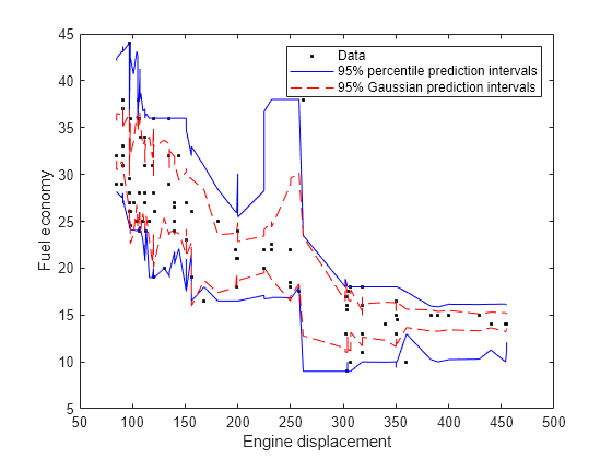
Perform quantile regression to predict the out-of-bag 2.5% and 97.5% percentiles.
oobQuantPredInts = oobQuantilePredict(Mdl,'Quantile',[0.025,0.975]);
oobQuantPredInts
is an n
-by-2 numeric matrix of prediction intervals corresponding to the out-of-bag observations in Mdl.X
. n
is number of observations, size(Mdl.X,1)
. The first column contains the 2.5% percentiles and the second column contains the 97.5% percentiles.
Plot the observations and the estimated medians on the same figure. Compare the percentile prediction intervals and the 95% prediction intervals, assuming the conditional distribution of MPG
is Gaussian.
[oobMeanMPG,oobSTEMeanMPG] = oobPredict(Mdl); STDNPredInts = oobMeanMPG + [-1 1]*norminv(0.975).*oobSTEMeanMPG; [sX,idx] = sort(Mdl.X); figure; h1 = plot(Displacement,MPG,'k.'); hold on h2 = plot(sX,oobQuantPredInts(idx,:),'b'); h3 = plot(sX,STDNPredInts(idx,:),'r--'); ylabel('Fuel economy'); xlabel('Engine displacement'); legend([h1,h2(1),h3(1)],{'Data','95% percentile prediction intervals',... '95% Gaussian prediction intervals'}); hold off;
Estimate Out-of-Bag Conditional Cumulative Distribution Using Quantile Regression
Load the carsmall
data set. Consider a model that predicts the fuel economy of a car (in MPG) given its engine displacement.
load carsmall
Train an ensemble of bagged regression trees using the entire data set. Specify 100 weak learners and save the out-of-bag indices.
rng(1); % For reproducibility Mdl = TreeBagger(100,Displacement,MPG,'Method','regression',... 'OOBPrediction','on');
Estimate the out-of-bag response weights.
[~,YW] = oobQuantilePredict(Mdl);
YW
is an n-by-n sparse matrix containing the response weights. n
is the number of training observations, numel(Y)
. The response weights for the observation in Mdl.X(j,:)
are in YW(:,j)
. Response weights are independent of any specified quantile probabilities.
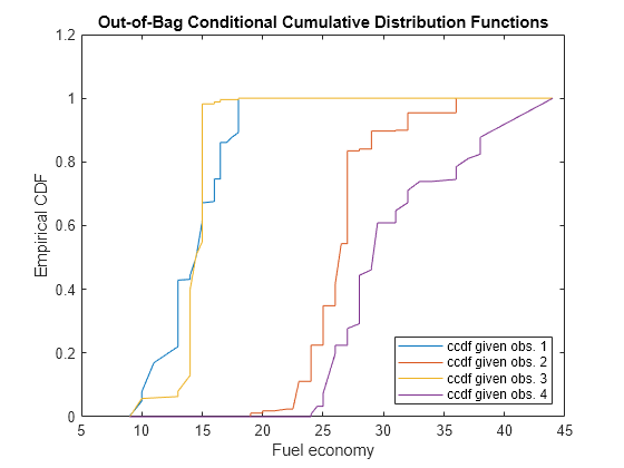
Estimate the out-of-bag, conditional cumulative distribution function (ccdf) of the responses by:
Sorting the responses is ascending order, and then sorting the response weights using the indices induced by sorting the responses.
Computing the cumulative sums over each column of the sorted response weights.
[sortY,sortIdx] = sort(Mdl.Y); cpdf = full(YW(sortIdx,:)); ccdf = cumsum(cpdf);
ccdf(:,j)
is the empirical out-of-bag ccdf of the response, given observation j
.
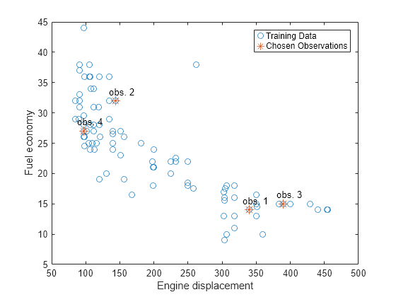
Choose a random sample of four training observations. Plot the training sample and identify the chosen observations.
[randX,idx] = datasample(Mdl.X,4); figure; plot(Mdl.X,Mdl.Y,'o'); hold on plot(randX,Mdl.Y(idx),'*','MarkerSize',10); text(randX-10,Mdl.Y(idx)+1.5,{'obs. 1' 'obs. 2' 'obs. 3' 'obs. 4'}); legend('Training Data','Chosen Observations'); xlabel('Engine displacement') ylabel('Fuel economy') hold off
Plot the out-of-bag ccdf for the four chosen responses in the same figure.
figure; plot(sortY,ccdf(:,idx)); legend('ccdf given obs. 1','ccdf given obs. 2',... 'ccdf given obs. 3','ccdf given obs. 4',... 'Location','SouthEast') title('Out-of-Bag Conditional Cumulative Distribution Functions') xlabel('Fuel economy') ylabel('Empirical CDF')
More About
Out-of-Bag
In a bagged ensemble, observations are out-of-bag when they are left out of the training sample for a particular learner. Observations are in-bag when they are used to train a particular learner.
When bagging learners, a practitioner takes a bootstrap sample (that is, a random sample with replacement) of size n for each learner, and then trains the learners using their respective bootstrap samples. Drawing n out of n observations with replacement omits on average about 37% of observations for each learner.
The out-of-bag ensemble error, the ensemble error estimated using out-of-bag observations only, is an unbiased estimator of the true ensemble error.
Quantile Random Forest
Quantile random forest [2] is a quantile-regression method that uses a random forest [1] of regression trees to model the conditional distribution of a response variable, given the value of predictor variables. You can use a fitted model to estimate quantiles in the conditional distribution of the response.
Besides quantile estimation, you can use quantile regression to estimate prediction intervals or detect outliers. For example:
To estimate 95% quantile prediction intervals, estimate the 0.025 and 0.975 quantiles.
To detect outliers, estimate the 0.01 and 0.99 quantiles. All observations smaller than the 0.01 quantile and larger than the 0.99 quantile are outliers. All observations that are outside the interval [L,U] can be considered outliers:
and
where:
Q1 is the 0.25 quantile.
Q3 is the 0.75 quantile.
IQR = Q3 – Q1 (the interquartile range).
Response Weights
Response weights are scalars that represent the conditional distribution of the response given a value in the predictor space. The observations in the bootstrap samples and the leaves that the training and test observations share induce response weights.
Given the observation x, the response weight for observation j in the training sample using tree t in the ensemble is
where:
I{h} is the indicator function.
St(x) is the leaf of tree t containing x.
ntrain is the number of training observations.
In other words, the response weights of a particular tree form the conditional relative frequency distribution of the response.
The response weights for the entire ensemble are averaged over the trees:
Algorithms
oobQuantilePredict
estimates out-of-bag quantiles
by applying quantilePredict
to all observations in the
training data (Mdl.X
). For each observation, the
method uses only the trees for which the observation is out-of-bag.
For observations that are in-bag for all trees in the ensemble, oobQuantilePredict
assigns
the sample quantile of the response data. In other words, oobQuantilePredict
does
not use quantile regression for out-of-bag observations. Instead,
it assigns quantile(Mdl.Y,
,
where tau
)tau
is the value of the Quantile
name-value
pair argument.
References
[1] Meinshausen, N. “Quantile Regression Forests.” Journal of Machine Learning Research, Vol. 7, 2006, pp. 983–999.
[2] Breiman, L. “Random Forests.” Machine Learning. Vol. 45, 2001, pp. 5–32.
Version History
Introduced in R2016b
Commande MATLAB
Vous avez cliqué sur un lien qui correspond à cette commande MATLAB :
Pour exécuter la commande, saisissez-la dans la fenêtre de commande de MATLAB. Les navigateurs web ne supportent pas les commandes MATLAB.
Select a Web Site
Choose a web site to get translated content where available and see local events and offers. Based on your location, we recommend that you select: .
You can also select a web site from the following list:
How to Get Best Site Performance
Select the China site (in Chinese or English) for best site performance. Other MathWorks country sites are not optimized for visits from your location.
Americas
- América Latina (Español)
- Canada (English)
- United States (English)
Europe
- Belgium (English)
- Denmark (English)
- Deutschland (Deutsch)
- España (Español)
- Finland (English)
- France (Français)
- Ireland (English)
- Italia (Italiano)
- Luxembourg (English)
- Netherlands (English)
- Norway (English)
- Österreich (Deutsch)
- Portugal (English)
- Sweden (English)
- Switzerland
- United Kingdom (English)