Solve Differential Algebraic Equations (DAEs)
This example show how to solve differential algebraic equations (DAEs) by using MATLAB® and Symbolic Math Toolbox™.
Differential algebraic equations involving functions, or state variables, , have the form
where is the independent variable. The number of equations must match the number of state variables .
Because most DAE systems are not suitable for direct input to MATLAB solvers, such as ode15i, first convert them to a suitable form by using Symbolic Math Toolbox functionality. This functionality reduces the differential index (number of differentiations needed to reduce the system to ODEs) of the DAEs to 1 or 0, and then converts the DAE system to numeric function handles suitable for MATLAB solvers. Then, use MATLAB solvers, such as ode15i, ode15s, or ode23t, to solve the DAEs.
Solve your DAE system by completing these steps.
Step 1: Specify Equations and Variables
The following figure shows the DAE workflow by solving the DAEs for a pendulum.
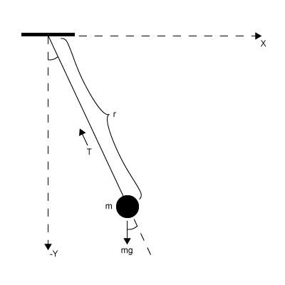
The state variables are:
Horizontal position of pendulum
Vertical position of pendulum
Tension force on pendulum string
The other variables are:
Pendulum mass
Pendulum length
Gravitational constant
The DAE system of equations is:
Specify independent variables and state variables by using syms.
syms x(t) y(t) T(t) m r g
Specify equations by using the == operator.
eqn1 = m*diff(x(t),2) == T(t)/r*x(t);
eqn2 = m*diff(y(t),2) == T(t)/r*y(t) - m*g;
eqn3 = x(t)^2 + y(t)^2 == r^2;
eqns = [eqn1 eqn2 eqn3];
Place the state variables in a column vector. Store the number of original variables for reference.
vars = [x(t); y(t); T(t)];
origVars = length(vars);
Step 2: Reduce Differential Order
2.1 (Optional) Check Incidence of Variables
This step is optional. You can check where variables occur in the DAE system by viewing the incidence matrix. This step finds any variables that do not occur in your input and can be removed from the vars vector.
Display the incidence matrix by using incidenceMatrix. The output of incidenceMatrix has a row for each equation and a column for each variable. Because the system has three equations and three state variables, incidenceMatrix returns a 3-by-3 matrix. The matrix has 1s and 0s, where 1s represent the occurrence of a state variable. For example, the 1 in position (2,3) means the second equation contains the third state variable T(t).
M = incidenceMatrix(eqns,vars)
M = 3×3

     1     0     1
     0     1     1
     1     1     0
If a column of the incidence matrix is all 0s, then that state variable does not occur in the DAE system and should be removed.
2.2 Reduce Differential Order
The differential order of a DAE system is the highest differential order of its equations. To solve DAEs using MATLAB, the differential order must be reduced to 1. Here, the first and second equations have second-order derivatives of x(t) and y(t). Thus, the differential order is 2.
Reduce the system to a first-order system by using reduceDifferentialOrder. The reduceDifferentialOrder function substitutes derivatives with new variables, such as Dxt(t) and Dyt(t). The right side of the expressions in eqns is 0.
[eqns,vars] = reduceDifferentialOrder(eqns,vars)
eqns =
vars =
Step 3: Check and Reduce Differential Index
3.1 Check Differential Index of System
Check the differential index of the DAE system by using isLowIndexDAE. If the index is 0 or 1, then isLowIndexDAE returns logical 1 (true) and you can skip step 3.2 and go to Step 4. Convert DAE Systems to MATLAB Function Handles. Here, isLowIndexDAE returns logical 0 (false), which means the differential index is greater than 1 and must be reduced.
isLowIndexDAE(eqns,vars)
ans = logical
   0
3.2 Reduce Differential Index with reduceDAEIndex
To reduce the differential index, the reduceDAEIndex function adds new equations that are derived from the input equations, and then replaces higher-order derivatives with new variables. If reduceDAEIndex fails and issues a warning, then use the alternative function reduceDAEToODE as described in the workflow Solve Semilinear DAE System.
Reduce the differential index of the DAEs described by eqns and vars.
[DAEs,DAEvars] = reduceDAEIndex(eqns,vars)
DAEs =
DAEvars =
If reduceDAEIndex issues an error or a warning, use the alternative workflow described in Solve Semilinear DAE System.
Often, reduceDAEIndex introduces redundant equations and variables that can be eliminated. Eliminate redundant equations and variables using reduceRedundancies.
[DAEs,DAEvars] = reduceRedundancies(DAEs,DAEvars)
DAEs =
DAEvars =
Check the differential index of the new system. Now, isLowIndexDAE returns logical 1 (true), which means that the differential index of the system is 0 or 1.
isLowIndexDAE(DAEs,DAEvars)
ans = logical
   1
Step 4: Convert DAE Systems to MATLAB Function Handles
This step creates function handles for the MATLAB ODE solver ode15i, which is a general purpose solver. To use specialized mass matrix solvers such as ode15s and ode23t, see Solve DAEs Using Mass Matrix Solvers and Choose an ODE Solver.
reduceDAEIndex outputs a vector of equations in DAEs and a vector of variables in DAEvars. To use ode15i, you need a function handle that describes the DAE system.
First, the equations in DAEs can contain symbolic parameters that are not specified in the vector of variables DAEvars. Find these parameters by using setdiff on the output of symvar from DAEs and DAEvars.
pDAEs = symvar(DAEs);
pDAEvars = symvar(DAEvars);
extraParams = setdiff(pDAEs,pDAEvars)
extraParams =
The extra parameters that you need to specify are the mass m, radius r, and gravitational constant g.
Create the function handle by using daeFunction. Specify the extra symbolic parameters as additional input arguments of daeFunction.
f = daeFunction(DAEs,DAEvars,g,m,r);
The rest of the workflow is purely numerical. Set the parameter values and create the function handle for ode15i.
gVal = 9.81;
mVal = 1;
rVal = 1;
F = @(t,Y,YP) f(t,Y,YP,gVal,mVal,rVal);
Step 5: Find Initial Conditions for Solvers
The ode15i solver requires initial values for all variables in the function handle. Find initial values that satisfy the equations by using the MATLAB decic function. decic accepts guesses (which might not satisfy the equations) for the initial conditions and tries to find satisfactory initial conditions using those guesses. decic can fail, in which case you must manually supply consistent initial values for your problem.
First, check the variables in DAEvars.
DAEvars
DAEvars =
Here, Dxt(t) is the first derivative of x(t), Dytt(t) is the second derivative of y(t), and so on. There are 7 variables in a 7-by-1 vector. Therefore, guesses for initial values of variables and their derivatives must also be 7-by-1 vectors.
Assume the initial angular displacement of the pendulum is 30° or pi/6, and the origin of the coordinates is at the suspension point of the pendulum. Given that we used a radius rVal of 1, the initial horizontal position x(t) is rVal*sin(pi/6). The initial vertical position y(t) is -rVal*cos(pi/6). Specify these initial values of the variables in the vector y0est.
Arbitrarily set the initial values of the remaining variables and their derivatives to 0. These are not good guesses. However, they suffice for this problem. In your problem, if decic errors, then provide better guesses and refer to decic.
y0est = [rVal*sin(pi/6); -rVal*cos(pi/6); 0; 0; 0; 0; 0];
yp0est = zeros(7,1);
Create an option set that specifies numerical tolerances for the numerical search.
opt = odeset(RelTol=1e-7,AbsTol=1e-7);
Find consistent initial values for the variables and their derivatives by using decic.
[y0,yp0] = decic(F,0,y0est,[],yp0est,[],opt)
y0 = 7×1

    0.4771
   -0.8788
   -8.6214
         0
   -0.0000
   -2.2333
   -4.1135
yp0 = 7×1

         0
   -0.0000
         0
         0
   -2.2333
         0
         0
Step 6: Solve DAEs Using ode15i
Solve the system integrating over the time span 0 ≤ t ≤ 0.5. Add the grid lines and the legend to the plot.
[tSol,ySol] = ode15i(F,[0 0.5],y0,yp0,opt);
plot(tSol,ySol(:,1:origVars),LineWidth=2)

for k = 1:origVars
  S{k} = char(DAEvars(k));
end

legend(S,Location="best")
grid on

Solve the system for different parameter values by setting the new value and regenerating the function handle and initial conditions.
Set rVal to 2 and regenerate the function handle and initial conditions.
rVal = 2;
F = @(t,Y,YP) f(t,Y,YP,gVal,mVal,rVal);

y0est = [rVal*sin(pi/6); -rVal*cos(pi/6); 0; 0; 0; 0; 0];
[y0,yp0] = decic(F,0,y0est,[],yp0est,[],opt);
Solve the system for the new parameter value.
[tSol,y] = ode15i(F,[0 0.5],y0,yp0,opt);
plot(tSol,y(:,1:origVars),LineWidth=2)

for k = 1:origVars
  S{k} = char(DAEvars(k));
end
legend(S,Location="best")
grid on
