UAV Navigation in Unknown Environment with 2D Lidar SLAM

In the Improve UAV Position Estimation with Kalman Filter example, you learned a the method of estimating the position of a UAV within a known map of the environment, and its importance in autonomous navigation.

However, in real life scenarios, equipping UAVs with a known map of the environment is not always possible because you might not know the environment itself beforehand. For example, UAVs used to survey natural disaster sites must create maps of the disaster aftermath as they fly, and UAVs that inspect buildings also need to map the buildings during their missions.

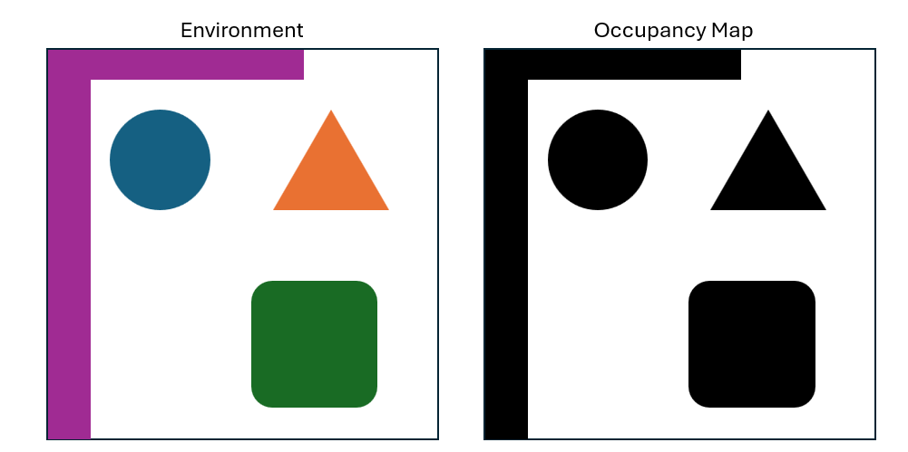
You can use occupancy maps to represent obstacles in the environment. In an occupancy map, each cell has an assigned value from 0 to 1. Cells with values closer to 0 have a lighter shade, indicating regions that have a lower probability of containing an obstacle, while cells with values closer to 1 have a darker shade, indicating regions with a higher probability of containing obstacles.

Introduction to Lidar Sensors

One method of mapping obstacles in the environment is to equip the UAV with a lidar sensor. Lidar stands for "light detection and ranging". The sensor works by emitting laser pulses that reflect off the surrounding obstacles. The sensor then detects the reflected light and calculates the distance to the obstacle that reflected it based on the time required for the reflection to reach the sensor. The sensor stores the obstacle it detects as point clouds.

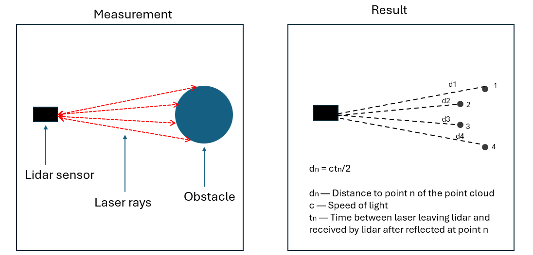
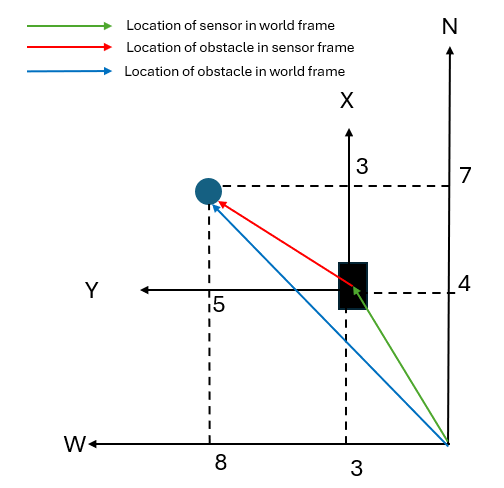
Lidar point cloud data provides information on the position of a detected obstacle relative to the sensor in the sensor frame. By combining the point cloud data with the lidar sensor orientation and position in the world frame, you can obtain the position of the obstacle in the world frame and use it to build a map of the environment.

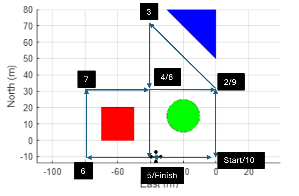
For example, if a lidar sensor that faces north detects obstacles at 3 meters in the *x-*direction and 5 meters in the *y-*direction of the sensor frame, and that sensor is located 4 meters north and 3 meters west of the world frame origin, then the obstacles are located 7 meters north and 8 meters west of the world frame origin.

Simulate 2D UAV Obstacle Mapping with Lidar Sensor

To illustrate the process, simulate a simple UAV scenario. In the simulation, the UAV is equipped with lidar sensor. The UAV is also equipped with GPS sensor which provides the estimated position of the UAV and lidar sensor in world frame.

To simplify the simulation, the UAV is configured to have a constant orientation of 0 degrees pitch, roll, and yaw, The lidar sensor also has a 360 degree lidar sensors which allows the sensor to capture its surrounding without having to change its orientations.

First create a UAV scenario with an update rate of 1Hz.

scene = uavScenario(UpdateRate=1); 

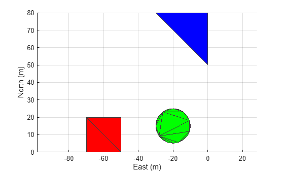
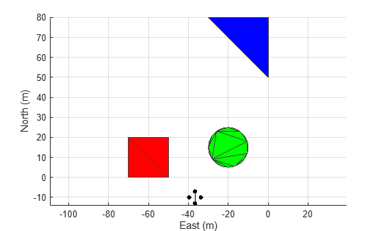
Add three meshes in the scenario to represent obstacles, and show the scene

% Obstacle 1
addMesh(scene,"Polygon",{[-70 0;-50 0;-50 20;-70 20],[0 40]},[1 0 0]); 
% Obstacle 2
addMesh(scene,"cylinder",{[-20 15 10],[0 60]},[0 1 0]);  
% Obstacle 3
addMesh(scene,"Polygon",{[0 50;0 80;-30 80],[0 50]},[0 0 1]); 

show3D(scene);
view([0 90])
axis equal
grid on

Run the generateUAVMotionHelper script to generate a motion vector for the UAV. The motion vector contains the positions, orientations, velocities, and accelerations of the UAV that navigate the UAV around the obstacles.

generateUAVMotionHelper

Create a UAV platform, and assign a quadcopter mesh to the platform.

plat = uavPlatform("UAV",scene,ReferenceFrame="ENU", ...
       InitialPosition=flightPositions(1,:), ...
       InitialOrientation=flightOrientation(1,:), ...
       InitialVelocity=flightVelocity(1,:)); 

updateMesh(plat,"quadrotor",{8},[0 0 0],eye(4))

Create a lidar sensor by using the uavLidarPointCloudGenerator object, which generates a 3D lidar scan reading. To simulate a 2D lidar sensor, specify an elevation limit of 0 degrees.

lidarmodel = uavLidarPointCloudGenerator(AzimuthLimits=[-180 180], ...
             AzimuthResolution=0.6,ElevationLimits=[0 0], ...
             ElevationResolution=2.5,MaxRange=100,RangeAccuracy=0.002, ...
             UpdateRate=1, ...
             HasOrganizedOutput=true);

Attach the sensor to the UAV platform.

lidar = uavSensor("Lidar",plat,lidarmodel, ...
        MountingLocation=[0 0 -1],MountingAngles=[0 0 0]); 

Create a GPS sensor and attach the sensor to the UAV.

gpsmodel = gpsSensor(UpdateRate=1,DecayFactor=0.1, ...
           RandomStream="mt19937ar with seed",Seed=10, ...
           HorizontalPositionAccuracy=2, ...
           ReferenceFrame="ENU");

gps = uavSensor("GPS",plat,gpsmodel); 

Initialize a cell array in which to store lidar scan data and an empty vector in which to store pose data.

lidarScanData = cell(1,size(flightMotion,1));
lidarPoseData = zeros([size(flightMotion,1) 3]);

Set up the scene visualization, and prepare the UAV scenario for visualization.

[ax,plotFrames] = show3D(scene);
view([0 90]);
grid on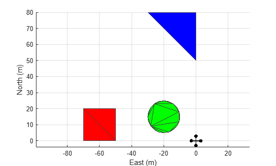

setup(scene)

Start the simulation. In each step of the simulation:

1. Read the lidar sensor data.

2. Read the GPS sensor data.

3. Obtain the lidar sensor orientation angle.

4. Construct and store a lidar sensor pose vector that consists of a GPS position and a lidar sensor orientation.

5. Remove invalid lidar scan points.

6. Convert the lidar scan to 2D by extracting only the x- and y-coordinates of the scan.

7. Store the lidar scan data.

8. Visualize the UAV scenario.

9. Advance the UAV scenario, move the UAV to the next position, and update the sensors.

for ptIdx = 1:size(flightMotion,1)
    % Read the lidar sensor data
    [~,lidarSampleTime,lidarSensorReading] = read(lidar);

    % Read the GPS sensor data
    [~,~,gpsread] = read(gps);
    gpspos = lla2enu(gpsread,[0 0 0],"flat");

    % Obtain lidar sensor orientation angle
    lidarTransform = getTransform(scene.TransformTree,"ENU","UAV/Lidar",lidarSampleTime);
    lidarAngle = tform2eul(lidarTransform);
    lidarZangle = lidarAngle(1);

    % Construct and store lidar sensor pose vector
    lidarSensorPose = [gpspos(1:2) lidarZangle];
    lidarPoseData(ptIdx,:) = lidarSensorPose;

    % Remove invalid lidar scan points
    lidarSensorReading = removeInvalidPoints(lidarSensorReading);

    % Extract only the x- and y-coordinates of the scan
    lidarSensorReading2D = lidarSensorReading.Location(:,(1:2));

    % Store lidar scan data
    lidarScanData(ptIdx) = {lidarScan(lidarSensorReading2D)};
    
    % Visualize UAV scenario
    show3D(scene,Time=lidarSampleTime,FastUpdate=true,Parent=ax);
    view([0 90]);
    axis equal
    grid on
    refreshdata
    drawnow limitrate

    % Advance scenario, move UAV to next position, and update sensors
    advance(scene);
    move(plat,flightMotion(ptIdx,:))
    updateSensors(scene)
end

Construct Occupancy Map with Lidar and GPS Data

Use the buildMap function to construct the occupancy map. The function constructs the map by placing the lidar scans contained in the lidarScanData vector in the positions and orientations contained in the lidarPoseData vector.

occMap = buildMap(lidarScanData,lidarPoseData,5,lidarmodel.MaxRange);
show(occMap)
axis equal
xlim([-125 55])
ylim([-25 80])
title("Occupancy Map with Lidar and GPS Data")

Notice that this occupancy map is not a good representation of the environment because it does not clearly define regions in which obstacles are present. If a UAV were to use this map for autonomous navigation, it would risk colliding with obstacles since it would not be able to accurately determine its position relative to the obstacles.

If you could construct the occupancy map with perfect knowledge of the lidar sensor position, orientation, and range measurement, then the resulting occupancy map would show a perfect representation of the environment. However, as in real life scenarios, the sensors you have used up to this point have limited accuracy:

1. The range measured by the lidar sensor, which provides the positions of the obstacles relative to the UAV, has random errors with a standard deviation of 0.002 meters.

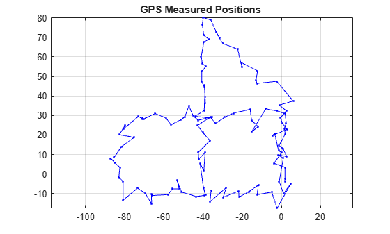
2. The horizontal position measured by the GPS sensor, which provides the position of the UAV and lidar sensor, has a random error with a standard deviation of 2 meters. This plot shows the positions measured by the GPS, which are noisy and corrupt the occupancy map.

plot(lidarPoseData(:,1),lidarPoseData(:,2),Marker=".",Color="b")
grid on
axis equal
title("GPS Measured Positions ")

Simultaneous Localization and Mapping

The poor quality of your occupancy map illustrates the challenge addressed by the of simultaneous localization and mapping (SLAM) algorithm:

To create an accurate map of its environment, a UAV must accurately localize its position in the world frame and relative to obstacle. However, to accurately localize its position in the world frame and relative to obstacles, a UAV must have an accurate map of the environment.

The simultaneous localization and mapping (SLAM) algorithm addresses this paradox by building a map of the environment as it localizes the position of the UAV within that map.

This example focuses on 2D lidar SLAM algorithm that uses pose graph optimization to estimate the UAV trajectory by using the complete set of measurements. This algorithm also has the benefit of not requiring additional sensors, such as GPS, which makes it suitable for UAV missions in which GPS signals are not available or inaccurate such as indoor flights or flights near tall buildings.

Introduction to 2D Lidar SLAM with Scan Matching and Loop Closure

A pose graph consist of nodes that represents the pose (consisting of the location and orientation) of the lidar sensor and edges that represent the distance between each pose. An accurate pose graph enables you to determine the location and orientation of the lidar sensor (and therefore, the UAV) at each step of the mission, which is necessary to localize the UAV and to build a map of the environment.

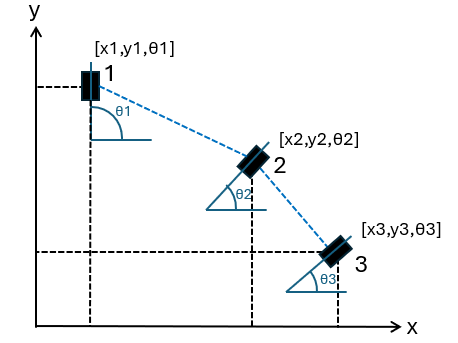
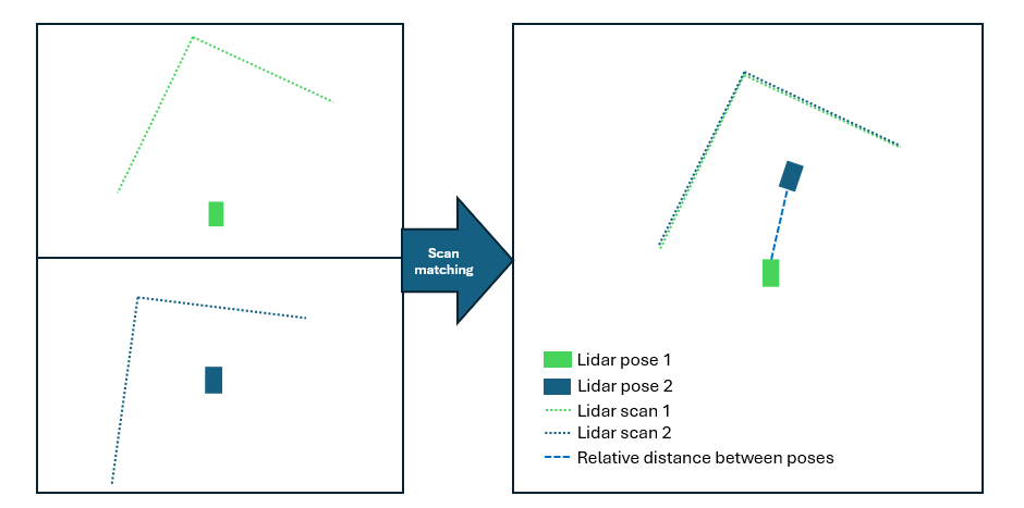
In this example, the pose of the lidar sensor is estimated using scan matching algorithm which estimates the relative pose between the lidar sensor poses where the scans were taken. The algorithm estimates the relative pose of each subsequent lidar scan this by using these steps:

1. Constrain each lidar sensor pose to its scan.

2. Analyze the current lidar scan against the previous scan to search for similar features in each pair of scans.

3. Transform the current lidar scan to align its matched features to the similar features in the previous scan.

4. Apply the transformation to the lidar sensor pose at the current scan to obtain the relative pose.

The process repeats for each subsequent scan to obtain the complete pose graph.

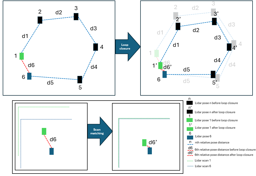
The example further refines the estimated poses by using loop closure. The loop-closure process begins when the algorithm detects that the current lidar scan measures the same part of the environment as one of the previous scans. At which point, the algorithm creates a pose loop and performs these steps:

1. Constrain the first and last lidar sensor poses in the loop to their respective scans.

2. Analyze the first lidar scan against the last scan in the loop to search for similar features.

3. Transform the last lidar scan in the loop to align its matched features to the similar features in the first scan.

4. Apply the transformation to the last lidar sensor pose while maintaining the distances between previous pairs of lidar sensor poses.

This process improves the position estimates of all poses in the loop.

Simulate 2D Lidar SLAM with Scan Matching and Loop Closure

To simulate 2D Lidar SLAM, first create a lidarSLAM (Navigation Toolbox) object with a map resolution of 5 cells per meter and the same maximum lidar range as the lidar sensor used in the scenario simulation.

slamObj = lidarSLAM(5,lidarmodel.MaxRange);

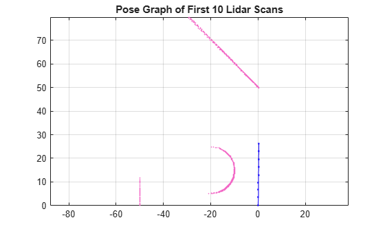
Add the first 10 lidar scans to the lidarSLAM object, and show the pose graph. Observe that, by aligning the edges of the square, circular, and triangular obstacles, the lidarSLAM object can estimate the pose of the lidar sensor for the first 10 scans.

for i = 1:10
    [isScanAccepted,loopClosureInfo,optimizationInfo] = addScan(slamObj,lidarScanData{i});
end
show(slamObj);
title("Pose Graph of First 10 Lidar Scans");

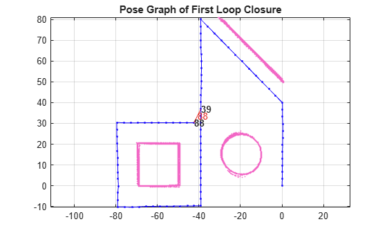
Continue adding lidar scans to the lidarSLAM object, using all of the scans gathered during the simulations. When the lidarSLAM object detects a loop closure, display the pose graph. Observe that, for the 88th lidar scan, the lidarSLAM object detects that the lidar sensor is in a similar location to when the sensor took the 39th scan, and starts performing the loop closure.

firstTimeLCDetected = false;
for i = 11:numel(lidarScanData)
    [isScanAccepted,loopClosureInfo,optimizationInfo] = addScan(slamObj,lidarScanData{i});
    if ~isScanAccepted
        continue
    end
    if optimizationInfo.IsPerformed && ~firstTimeLCDetected
        show(slamObj);
        hold on
        show(slamObj.PoseGraph); 
        axis equal
        hold off
        firstTimeLCDetected = true;
        drawnow
    end
end
title("Pose Graph of First Loop Closure");

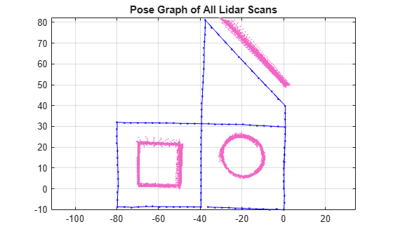
Show the pose graph that uses all the lidar scans. Observe that the scan-matching and loop-closure algorithm has produced a much more accurate lidar sensor pose estimate than the GPS sensor estimate.

show(slamObj);
axis equal
title("Pose Graph of All Lidar Scans")

Create a new occupancy map using the lidar sensor poses that you have optimized using lidar scan matching and loop closure.

[optScans,optPoses] = scansAndPoses(slamObj);
occMap = buildMap(optScans,optPoses,5,lidarmodel.MaxRange);
show(occMap);
axis equal
xlim([-125 55])
ylim([-25 90])
title("Occupancy Map with Scan Matching and Loop Closure")

Notice that the new occupancy map clearly defines the regions in which obstacles are present, providing a better representation of the environment. This map enables a UAV to safely plan an obstacle free-path. To learn how to use the generated occupancy map for motion planning that avoids obstacles, see the Motion Planning with RRT for Fixed-Wing UAV example.

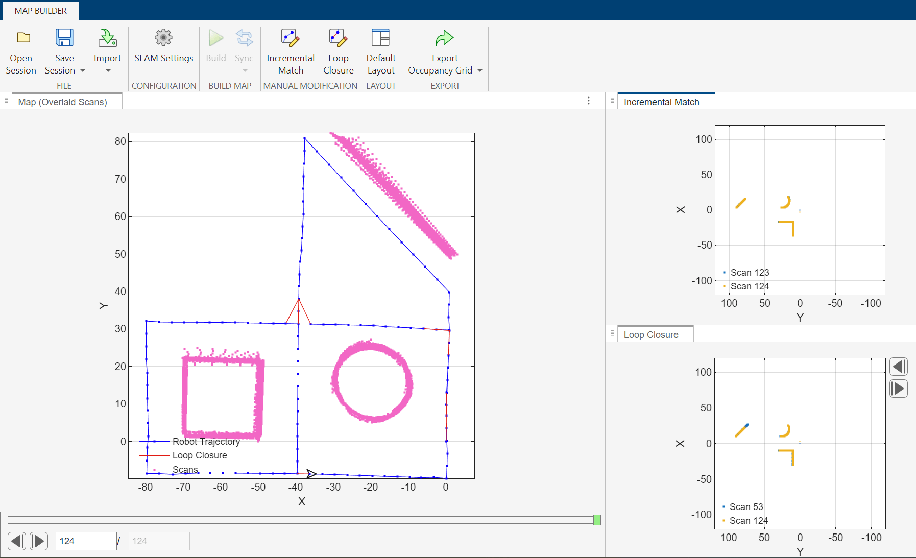
Simulate 2D Lidar SLAM using SLAM Map Builder App

You can also use the SLAM Map Builder app to simulate 2D lidar SLAM and create an optimized pose graph. To open the app, on the Apps tab of the MATLAB® Toolstrip, in the Robotics and Autonomous Systems section, select the SLAM Map Builder icon. Alternatively, enter slamMapBuilder in the Command Window.

Once the app is open, follow these steps to simulate 2D lidar SLAM:

1. In the app toolstrip, select Import, then Import from workspace. This opens the Import from Workspace tab.

2. In the Select Scans section of the toolstrip, set Scans to lidarScanData.

3. In the Select Poses (Odometry) section of the toolstrip, set Poses (Odometry) to lidarPoseData.

4. To import the scan and pose data, click Apply. Then, to return to the Map Builder tab, click Close Import.

5. In the Configuration section of the toolstrip, select SLAM Settings, and then specify these options:

   1. Map Resolution (cells/m) — 5

   2. Lidar Range [min,max] (m) — 0 100

6. Click OK to save the SLAM Settings, and then click Build to start the map building process.