Structure from Motion from Multiple Views

R2026b

Since R2026a

Structure from Motion (SfM) is a computer vision technique for estimating the 3-D structure of a scene from a collection of 2-D images [1]. It plays a critical role in applications such as robot navigation, autonomous driving, augmented reality, and 3-D scene reconstruction.

This example provides a comprehensive walkthrough of an incremental SfM pipeline, demonstrating how to estimate camera poses and reconstruct a 3-D scene from a set images from a calibrated camera.

Structure from Motion Pipeline Overview

This section offers a streamlined overview of the entire SfM workflow end-to-end using the sfm object and associated object functions. Use the following code example as a template to process your own image data or use sample datasets to reconstruct a 3-D scene with minimal setup.

% Initialize the sfm object with an image datastore and camera intrinsics
sfmObj = sfm(imds,intrinsics);

% Create a view graph by connecting visually similar image pairs
sfmObjViewGraph = connectImagePairs(sfmObj,Verbose=true);

% Verify the view graph by checking geometric consistency between image pairs
sfmObjVerified = verifyImagePairs(sfmObjViewGraph,Verbose=true);

% Triangulate an initial set of 3-D points from an image pair
sfmObjInit = triangulateInitialViews(sfmObjVerified,Verbose=true);

% Incrementally process views in the view graph to build the 3-D structure of the scene
sfmObjFinal = reconstruct(sfmObjInit,Verbose=true);

% Retrieve estimated camera poses of each image and the reconstructed 3-D points
camPoses = poses(sfmObjFinal);
sparsePoints = pointCloud(sfmObjFinal);

% Display the reconstructed scene showing camera positions and 3-D point cloud
plot(sfmObjFinal)

The rest of this example provides a detailed step-by-step walkthrough of running the structure-from-motion pipeline on an indoor scene, along with visualization, analysis and evaluation of results. For more information about best practices for using SfM to reconstruct 3-D scenes, see Best Practices for 3-D Reconstruction Using Structure from Motion.

Run SfM on the TUM RGB-D Benchmark Dataset

This section demonstrates how to run the full structure-from-motion pipeline using a subset of the TUM RGB-D Benchmark dataset [2].

Download the Dataset

You can download the data to a temporary directory using a web browser or by running the following code:

[imageFolder, downloadFolder] = helperDownloadTUMData;

Load Images and Camera Intrinsics

Create an imageDatastore to manage the images. The images are sequentially ordered in time, but the SfM pipeline demonstrated in this example also supports non-sequential images.

imds = imageDatastore(imageFolder);

This example uses images collected from a calibrated camera. To calibrate a camera, use the Using the Single Camera Calibrator App.

Load camera intrinsics parameters.

intrinsicsFile = fullfile(downloadFolder, "sfmTrainingDataTUMRGBD", "cameraInfo.mat");
data = load(intrinsicsFile);
intrinsics = data.intrinsics;

Visualize the first 25 images from the scene.

montage(imds, Size=[5 5])
title("Sample Images")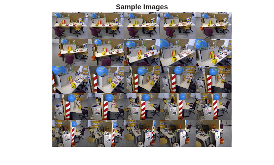

Create sfm object

Create the sfm object to manage data and operations required for Structure from Motion.

sfmObj = sfm(imds,intrinsics);

Connect Image Pairs and Build View Graph

This section shows how to build a view graph from a collection of images using bag-of-features similarity search. A view graph is a graph where each node represents an image and each edge indicates that two images are likely to see overlapping scene content. View graphs are used as a starting point for Structure from Motion and visual SLAM pipelines.

Use the connectImagePairs function to connect image pairs based on visual similarity. The values of NumSimilarImages and MatchThreshold are set to default values that work well on most datasets. Decrease the MatchThreshold value and increase the NumSimilarImages value for challenging cases to prevent the view graph from splitting into disconnected components. Refer to Display View Graph Created Using Visual Similarity Matching for details on analyzing these results.

sfmObjViewGraph = connectImagePairs(sfmObj,NumSimilarImages=10,MatchThreshold=40,Verbose=true);

Refine View Graph Using Geometric Verification

Appearance-based feature matching often proposes many candidate image pairs and putative correspondences. However, these matches can include a significant number of outliers due to repeated textures, illumination changes, or viewpoint differences. Use verifyImagePairs to filter these outlier pairs by enforcing projective geometry constraints. Ensure that the view graph was created successfully before proceeding to geometric verification. For challenging datasets, reduce MinNumInliers and increase MaxDistance to relax the geometric verification conditions and prevent most graph edges from being removed.

if isConnected(sfmObjViewGraph)
    sfmObjVerified = verifyImagePairs(sfmObjViewGraph,MinNumInliers=30,MaxDistance=4,Verbose=true);
end

393 out of 468 edges passed geometric verification.
Average 2D inliers count: 213.338422
Minimum 2D inliers count: 31
Maximum 2D inliers count: 681

Triangulate 3-D Points from Initial View Pair

Use triangulateInitialViews to select a robust image pair and initialize the 3-D reconstruction. The quality of this pair strongly affects the accuracy and runtime of subsequent stages because errors introduced here propagate through the pipeline. Strong initial pairs come from densely connected regions of the view graph, where both images share substantial scene overlap.

Confirm that geometric verification completed successfully before initializing the reconstruction. Specify a minimum median angle of 16 degrees and a maximum triangulation error of 4 pixels. Display the triangulation metrics.

if isVerified(sfmObjVerified)
    [sfmObjInit,info] = triangulateInitialViews(sfmObjVerified,MinMedianAngle=16,MaxTriangulationError=4,Verbose=true);
    disp(info)
end

277 of 393 edges have more than 100 feature matches.
265 of 277 edges are selected after applying the grid threshold.
Views 32 and 34 are selected for initial triangulation.
Median triangulation angle: 16.103256

                     ViewId1: 32
                     ViewId2: 34
                RelativePose: [1×1 rigidtform3d]
                     Matches: [161×2 uint32]
    MedianTriangulationAngle: 16.1033
       MeanReprojectionError: 0.5856

Reconstruct Complete 3-D Scene Using Incremental Structure from Motion

After initialization with two views, use reconstruct to process the remaining views and incrementally build the 3-D structure of the entire scene. The process of selecting the next best view is critical because each choice influences the stability and accuracy of all subsequent steps in the reconstruction. The candidates for the next best view are the unprocessed images that contain a sufficient number of triangulated 3-D points. The optimal choice reduces camera pose uncertainty and contributes well-conditioned points to the structure.

Once the next view is selected, the sfm object processes it using these steps:

• Pose Estimation: Estimate the pose of the next view by solving the Perspective-n-Point (PnP) problem using 2-D feature correspondences to known 3-D points.

• Triangulation: Triangulate new 3-D points using the point tracks containing the next view.

• Bundle Adjustment: Perform bundle adjustment to jointly refine the pose of the next view, the poses of views that share sufficient tracks with it, and all 3-D points observed by these views.

• Re-Triangulation: Triangulate additional 3-D points with refined camera poses after each bundle adjustment. The improved poses increase triangulation accuracy and allow additional tracks to meet quality criteria.

Confirm that initialization succeeded before running incremental reconstruction. This step can take several minutes on standard hardware configurations.

if isInitialized(sfmObjInit)
    sfmObjFinal = reconstruct(sfmObjInit,GlobalRefinementFrequency=10,MinNumInliers=10,Verbose=true);
end

Retrieve Structure-from-Motion Results

Retrieve the estimated camera poses and the sparse 3-D point cloud.

camPoses = poses(sfmObjFinal);
sparsePoints = pointCloud(sfmObjFinal);

Visualize 3-D Reconstruction and Camera Poses

Use plot to display the reconstructed scene showing the camera positions and reconstructed sparse 3-D point cloud.

figure
plot(sfmObjFinal,CameraSize=0.3,MarkerSize=25,ShowLabel=false)

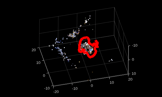
With the estimated camera poses and the sparse 3-D point cloud, you can perform dense reconstruction of the scene. See the following examples for more details on the dense reconstruction workflow:

• Dense 3-D Reconstruction from Multiple Views Using RAFT Optical Flow

• Reconstruct 3-D Scenes and Synthesize Novel Views Using Neural Radiance Field Model

Evaluate Estimated Camera Poses Against Ground Truth

metrics = compareTrajectories(camPoses, data.cameraPoses, AlignmentType="similarity");

disp("RMSE of absolute rotation (deg) = " + metrics.AbsoluteRMSE(1));

RMSE of absolute rotation (deg) = 1.107

disp("RMSE of absolute translation (m) = " + metrics.AbsoluteRMSE(2));

RMSE of absolute translation (m) = 0.010878

Visualize the absolute translation error.

figure
metrics.plot("absolute-translation")
view(0,0)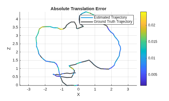

Visualize the absolute rotation error.

figure
metrics.plot("absolute-rotation")
view(0,0)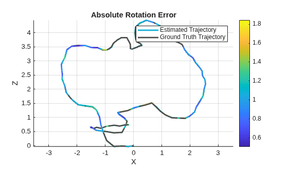

Visualize Intermediate Results of Structure from Motion

Inspect the intermediate results produced throughout the structure from motion pipeline to assess the quality of the reconstruction at each stage. Together, these visualizations provide insight into image connectivity, geometric verification, and the formation of the sparse 3-D reconstruction.

Display View Graph Created Using Visual Similarity Matching

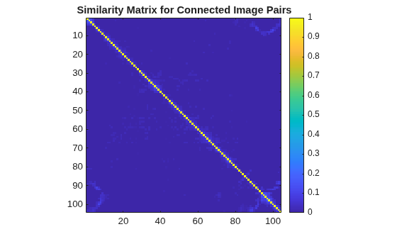
Visualize the similarity matrix for the connected image pairs using the imagesc function. A non-zero value at position (i,j) indicates that image i is connected to image j with a confidence score between 0 and 1. The dense blocks along the main diagonal correspond to the images with small camera motion and high scene overlap. This block structure is evident due to the sequential nature of the images being processed.

imagesc(sfmObjViewGraph.SimilarityMatrix)
colorbar
axis image
title("Similarity Matrix for Connected Image Pairs")

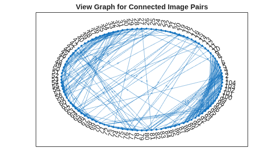
To assess overall connectivity, plot the nodes and edges in the view graph. A few long-range connections appear as outliers. Geometric verification prunes these outliers.

G = createPoseGraph(sfmObjViewGraph.ViewGraph);
figure
plot(G, NodeLabel=1:sfmObjViewGraph.NumImages, Layout="circle");
title("View Graph for Connected Image Pairs");

Display View Graph Refined Using Geometric Verification

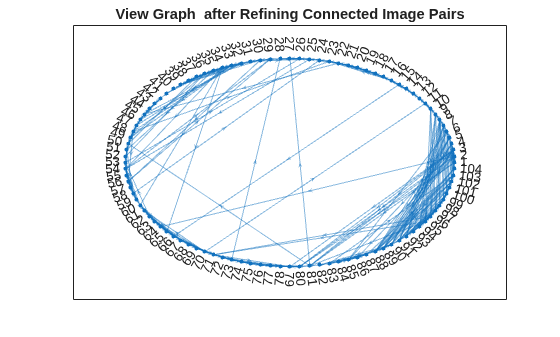
Plot the nodes and edges in the refined view graph. Observe that the number of spurious connections have been reduced compared to the initial view graph displayed in the previous section.

G1 = createPoseGraph(sfmObjVerified.ViewGraph);
figure
plot(G1, NodeLabel=1:sfmObjVerified.NumImages, Layout="circle");
title("View Graph after Refining Connected Image Pairs");

Display 3-D Reconstruction from Triangulating Initial View Pair

Visualize the initial image pair and matched keypoints.

I1 = readimage(imds, info.ViewId1);
I2 = readimage(imds, info.ViewId2);

points1 = sfmObjInit.ViewGraph.Views.Points{info.ViewId1};
points2 = sfmObjInit.ViewGraph.Views.Points{info.ViewId2};
matchedPoints1 = points1(info.Matches(:,1));
matchedPoints2 = points2(info.Matches(:,2));

figure
showMatchedFeatures(I1,I2,matchedPoints1,matchedPoints2,"montage",PlotOptions={"ro","g+","y--"})
title("View pair: "+num2str(info.ViewId1)+" and "+num2str(info.ViewId2))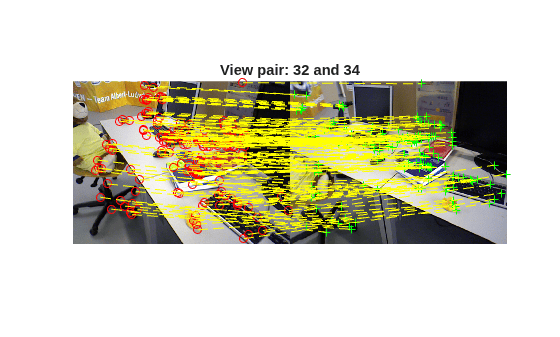

Visualize the triangulated 3-D points and the camera positions of the initial view pair.

figure
plot(sfmObjInit,CameraSize=0.5,ShowLabel=false,MarkerSize=25)
title("Triangulated points");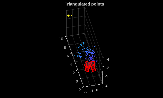

Inspect Incremental Reconstruction Statistics

Compare the number of processed images to the total number of images to ensure a complete reconstruction.

allImageIds = 1:sfmObjFinal.NumImages;
missedImages = setdiff(allImageIds, sfmObjFinal.ProcessedImages);
fprintf("Registered: %d / %d images.\n", ...
    numel(sfmObjFinal.ProcessedImages), sfmObjFinal.NumImages);

Registered: 104 / 104 images.

if ~isempty(missedImages)
    fprintf("Unregistered image IDs: %s\n", missedImages);
end

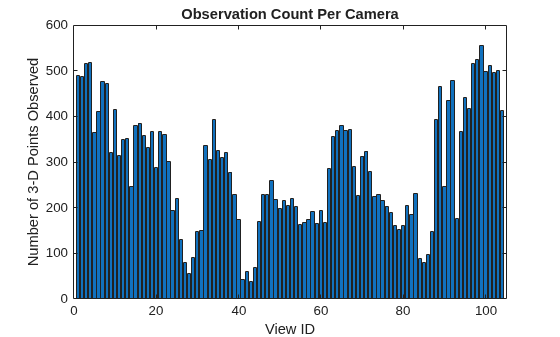
Determine how many 3-D points each registered view observes. The reconstruct function registers a view only when it finds at least 10 inlier correspondences between 2-D image features and known 3-D points. Views with observation counts near this threshold after reconstruction may have less reliable pose estimates. Increase the MinNumInliers value in the reconstruct function to enforce stricter registration criteria.

viewIds = sfmObjFinal.ProcessedImages;
obsCount = zeros(numel(viewIds), 1);
for i = 1:numel(viewIds)
    pts = findWorldPointsInView(sfmObjFinal.WorldPoints, viewIds(i));
    obsCount(i) = numel(pts);
end

figure
bar(viewIds, obsCount)
xlabel("View ID")
ylabel("Number of 3-D Points Observed")
title("Observation Count Per Camera")

Supporting Functions

helperDownloadTUMData

function [imageFolder, downloadFolder] = helperDownloadTUMData                                                                                                     
% Download and extract the TUM RGB-D dataset if not already present.                                                                                               
url = "https://ssd.mathworks.com/supportfiles/3DReconstruction/tum_rgbd_data.zip";                                                                                 
downloadFolder = tempdir;                                                                                                                                          
filename = fullfile(downloadFolder, "tum_rgbd_data.zip");                                                                                                          
imageFolder = fullfile(downloadFolder, "sfmTrainingDataTUMRGBD", "images");                                                                                        
if ~exist(imageFolder, "dir")                                                                                                                                      
    disp("Downloading TUM RGB-D Dataset (43 MB)...");                                                                                                              
    websave(filename, url);                                                                                                                                        
    unzip(filename, downloadFolder);                                                                                                                               
end                                                                                                                                                                
end 

References

[1] Schonberger, Johannes L., and Jan-Michael Frahm. "Structure-from-motion revisited." In Proceedings of the IEEE conference on computer vision and pattern recognition, pp. 4104-4113. 2016.

[2] Sturm, Jürgen, Nikolas Engelhard, Felix Endres, Wolfram Burgard, and Daniel Cremers. "A benchmark for the evaluation of RGB-D SLAM systems". In Proceedings of the IEEE/RSJ International Conference on Intelligent Robots and Systems, pp. 573-580, 2012.