Multivariate Wavelet Denoising

R2026b

The purpose of this example is to show the features of multivariate denoising provided in Wavelet Toolbox™.

Multivariate wavelet denoising problems deal with models of the form $X (t) = F (t) + e (t)$ , where the observation X is p-dimensional, F is the deterministic signal to be recovered, and e is a spatially-correlated noise signal. This example uses a number of noise signals and performs the following steps to denoise the deterministic signal.

This example uses noisy test signals. In this section, you will

Load a multivariate signal.
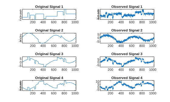
Display the original and observed signals.
Remove noise by a simple multivariate thresholding after a change of basis.
Display the original and denoised signals.
Improve the obtained result by retaining less principal components.
Display the number of retained principal components.
Display the estimated noise covariance matrix.

Load and Display Signal

Load a multivariate signal. Usually, only the matrix of data x is available. Here, we also have the true noise covariance matrix (covar) and the original signals (x_orig). These signals are noisy versions of simple combinations of the two original signals. The first one is “Blocks” which is irregular, and the second is “HeavySine,” which is regular except around time 750. The other two signals are the sum and the difference of the two original signals. Multivariate Gaussian white noise exhibiting strong spatial correlation is added to the resulting four signals, which leads to the observed data stored in x.

load ex4mwden
whos covar x x_orig

  Name           Size            Bytes  Class     Attributes

  covar          4x4               128  double              
  x           1024x4             32768  double              
  x_orig      1024x4             32768  double

Display the original and observed signals.

tiledlayout(4,2)
for k=1:4
    nexttile
    plot(x_orig(:,k))
    axis tight
    title("Original Signal "+num2str(k))
    nexttile
    plot(x(:,k))
    axis tight
    title("Observed Signal "+num2str(k))
end

The true covariance matrix is given by covar.

covar

covar = 4×4

    1.0000    0.8000    0.6000    0.7000
    0.8000    1.0000    0.5000    0.6000
    0.6000    0.5000    1.0000    0.7000
    0.7000    0.6000    0.7000    1.0000

Remove Noise by Simple Multivariate Thresholding

The denoising strategy combines univariate wavelet denoising in the basis where the estimated noise covariance matrix is diagonal with noncentered Principal Component Analysis (PCA) on approximations in the wavelet domain or with final PCA.

First, perform univariate denoising by setting the denoising parameters.

level = 5; 
wname = "sym4"; 
tptr  = "sqtwolog"; 
sorh  = "s";

Set the PCA parameters by retaining all the principal components.

npc_app = 4; 
npc_fin = 4;

Use wmulden to perform multivariate denoising.

x_den = wmulden(x, level, wname, npc_app, npc_fin, tptr, sorh);

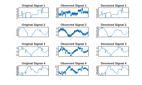
Display the original and denoised signals.

figure
tiledlayout(4,3)
for k = 1:4   
    nexttile
    plot(x_orig(:,k))
    xticks([])
    axis tight
    title("Original Signal "+num2str(k))
    nexttile
    plot(x(:,k))
    xticks([])
    axis tight
    title("Observed Signal "+num2str(k))
    nexttile
    plot(x_den(:,k))
    xticks([])
    axis tight
    title("Denoised Signal "+num2str(k))
end

Improve Results

Improve the first result by retaining fewer principal components.

The results are satisfactory. Focusing on the two first signals, note that they are correctly recovered, but the result can be improved by taking advantage of the relationships between the signals, leading to an additional denoising effect.

To automatically select the numbers of retained principal components by Kaiser's rule (which keeps the components associated with eigenvalues exceeding the mean of all eigenvalues), set npc_app and npc_fin both to "kais".

npc_app = 'kais'; 
npc_fin = 'kais';

Perform multivariate denoising again.

[x_den, npc, nestco] = wmulden(x, level, wname, npc_app, ...  
    npc_fin, tptr, sorh);

Display the number of retained principal components. The second output argument gives the numbers of retained principal components for PCA for approximations and for final PCA. As expected, since the signals are combinations of two initial ones, Kaiser's rule automatically detects that only two principal components are of interest.

npc

npc = 1×2

     2     2

Display the estimated noise covariance matrix. The third output argument contains the estimated noise covariance matrix. As you can see by comparing with the true matrix covar given previously, the estimation is satisfactory.

nestco

nestco = 4×4

    1.0784    0.8333    0.6878    0.8141
    0.8333    1.0025    0.5275    0.6814
    0.6878    0.5275    1.0501    0.7734
    0.8141    0.6814    0.7734    1.0967

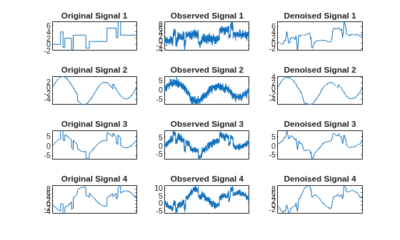
Display the original and final denoised signals. The results are better than those previously obtained. The first signal, which is irregular, is still correctly recovered, while the second signal, which is more regular, is denoised better after this second stage of PCA.

figure
tiledlayout(4,3)
for k = 1:4   
    nexttile
    plot(x_orig(:,k))
    xticks([])
    axis tight
    title("Original Signal "+num2str(k))
    nexttile
    plot(x(:,k))
    xticks([])
    axis tight
    title("Observed Signal "+num2str(k))
    nexttile
    plot(x_den(:,k))
    xticks([])
    axis tight
    title("Denoised Signal "+num2str(k))
end

Learning More About Multivariate Denoising

You can find more information about multivariate denoising, including some theory, simulations, and real examples, in the following reference:

M. Aminghafari, N. Cheze and J-M. Poggi (2006), "Multivariate denoising using wavelets and principal component analysis," Computational Statistics & Data Analysis, 50, pp. 2381-2398.