Accelerate BER Simulations of GMSK System Using FPGA-in-the-Loop Workflow

Since R2026a

This example shows how to accelerate bit error rate (BER) simulations of a Gaussian minimum shift keying (GMSK) communication system using FPGA-in-the-loop (FIL) workflow. In this example, you create a floating-point reference algorithm for a GMSK system using MATLAB®. After that you transition the algorithm into a fixed-point implementation using Simulink®, which ensures hardware compatibility and optimizes resource usage. Finally, you use the FIL workflow to generate HDL code and validate its BER performance on the AMD® Zynq UltraScale+™ MPSoC ZCU102 Evaluation Kit.

System Architecture

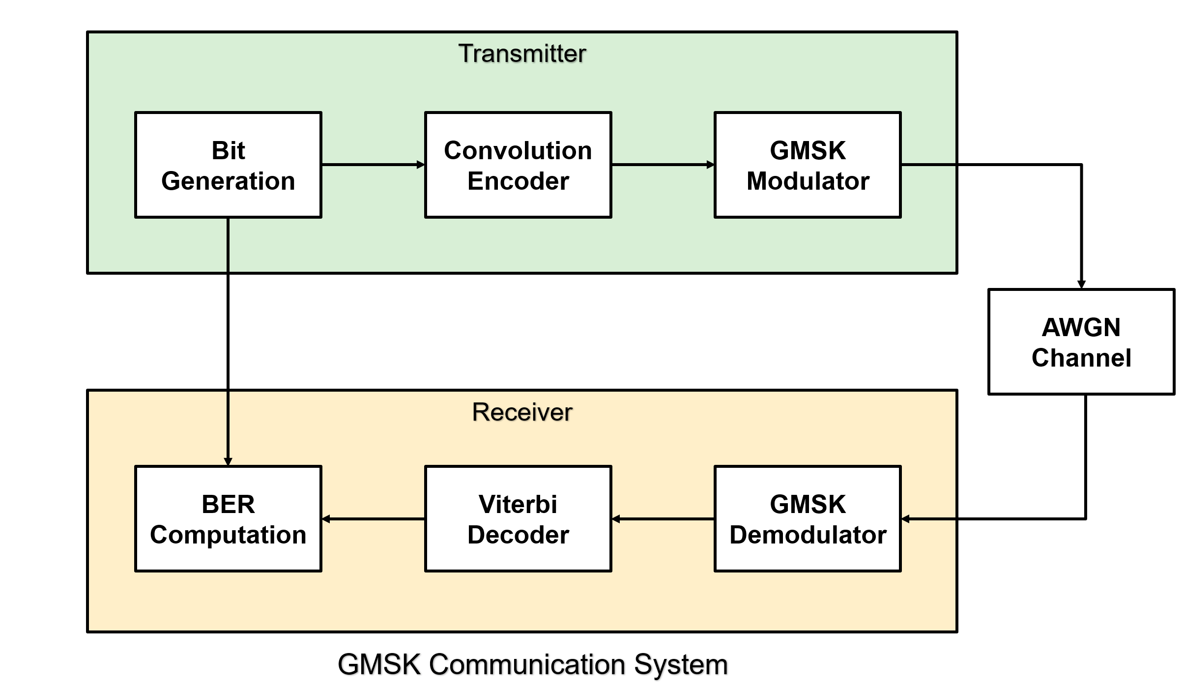
The following figure shows a high-level overview of a GMSK communication system. The system includes a convolutional encoder that adds redundancy for error correction, a GMSK modulator that provides bandwidth-efficient modulation with a constant envelope, and an additive white Gaussian noise (AWGN) channel that introduces noise. At the receiver, the system includes a GMSK demodulator that recovers the modulated signal and a Viterbi decoder that performs error correction.

Configure and Simulate Floating-Point Reference

You can configure and tune parameters interactively using Live Editor controls before running the simulation. The configurable parameters include constraint length, code generator polynomial, bandwidth time product, samples per symbol, pulse length, decision method, traceback depth, number of frames, and number of bits per frame.

constraintLength =  7;
codeGenerator = [171 133];
bandwidthTimeProduct = 0.3;
pulseLength = 1;
samplesPerSymbol = 2;
decisionMethod = 'Approximate log-likelihood ratio';
gmskTraceback = 16;
viterbiTraceback = 35;
numBitsPerFrame = 1000;
numFrames = 10;
EbNoVec = 0:10;
runBERonFPGA = false;

This example includes a script file, runGMSKML.m, to run the floating-point simulation. Running the script generates random data bits, applies convolutional encoding, and modulates the encoded bits using the GMSK modulator with the specified bandwidth-time product and pulse length. The modulated signal passes through the AWGN channel to introduce noise. At the receiver, the system demodulates the signal using the GMSK demodulator with the configured traceback length, and then decodes the data using the Viterbi decoder.

runGMSKML;

Implement Fixed-Point Model

This example includes a script file, runGMSKSL.m, to run the fixed-point Simulink simulation. This model replaces floating-point data types with fixed-point data types to prepare for hardware deployment. All the blocks in the Simulink model, GMSK Modulator, GMSK Demodulator, Convolutional Encoder, WGN Generator, and Viterbi Decoder are from Wireless HDL Toolbox™. These blocks provide optimized implementations of a GMSK modulator, GMSK demodulator, Convolutional encoder, WGN generator, and Viterbi decoder for HDL code generation. The model uses a ready signal at the output to control the input data flow, instead of using a multi-rate model, as shown in this figure.

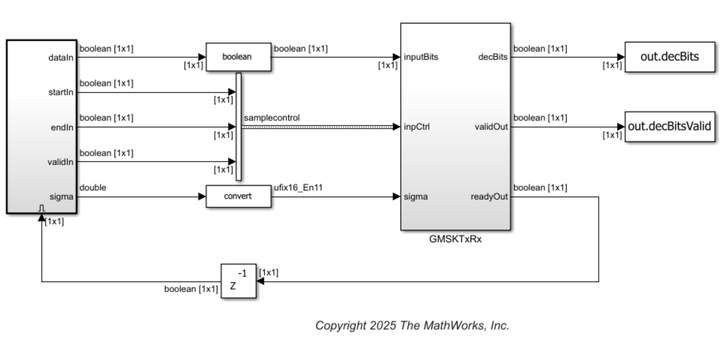
The GMSKTxRx subsystem comprises GMSK transmitter, AWGN, and GMSK receiver subsystems. The GMSKTxRx subsystem accepts data bits with sample control bus and the square root of noise variance as input, and provides decoded bits at the output with a corresponding valid signal. The ready signal at the output controls the input data flow without changing the sample rate.

Run the runGMSKSL script to run the Simulink model and get the BER curve for the Simulink model.

runGMSKSL;

For EbNo 0, BER is 0.419700
For EbNo 1, BER is 0.340000
For EbNo 2, BER is 0.221900
For EbNo 3, BER is 0.087500
For EbNo 4, BER is 0.029000
For EbNo 5, BER is 0.004100
For EbNo 6, BER is 0.000300
For EbNo 7, BER is 0.000000
For EbNo 8, BER is 0.000000
For EbNo 9, BER is 0.000000
For EbNo 10, BER is 0.000000
Elapsed time is 437.391994 seconds.

Generate HDL Code and Implement FIL

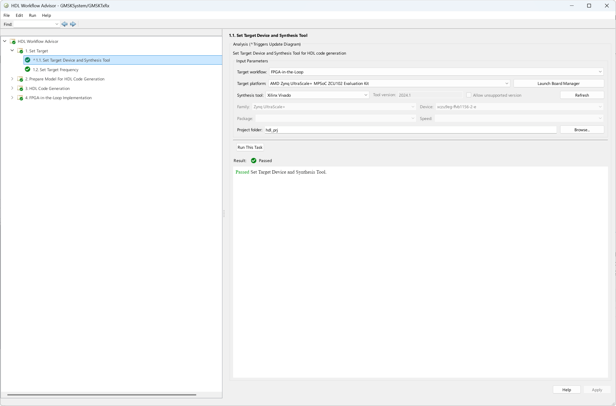
To generate HDL Code and implement FIL for this example, use HDL workflow advisor and set Target workflow to FPGA-in-the-loop and Target platform to AMD Zynq UltraScale+ MPSoC ZCU102 Evaluation kit.

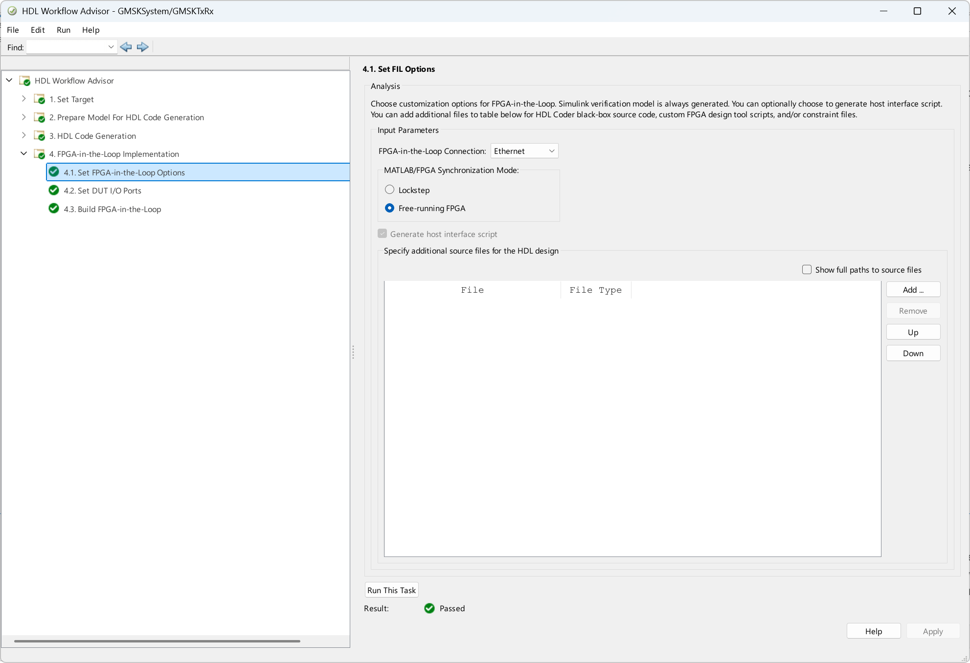
Generate HDL code and then, under MATLAB/FPGA Synchronization Mode, select Free-running FPGA.

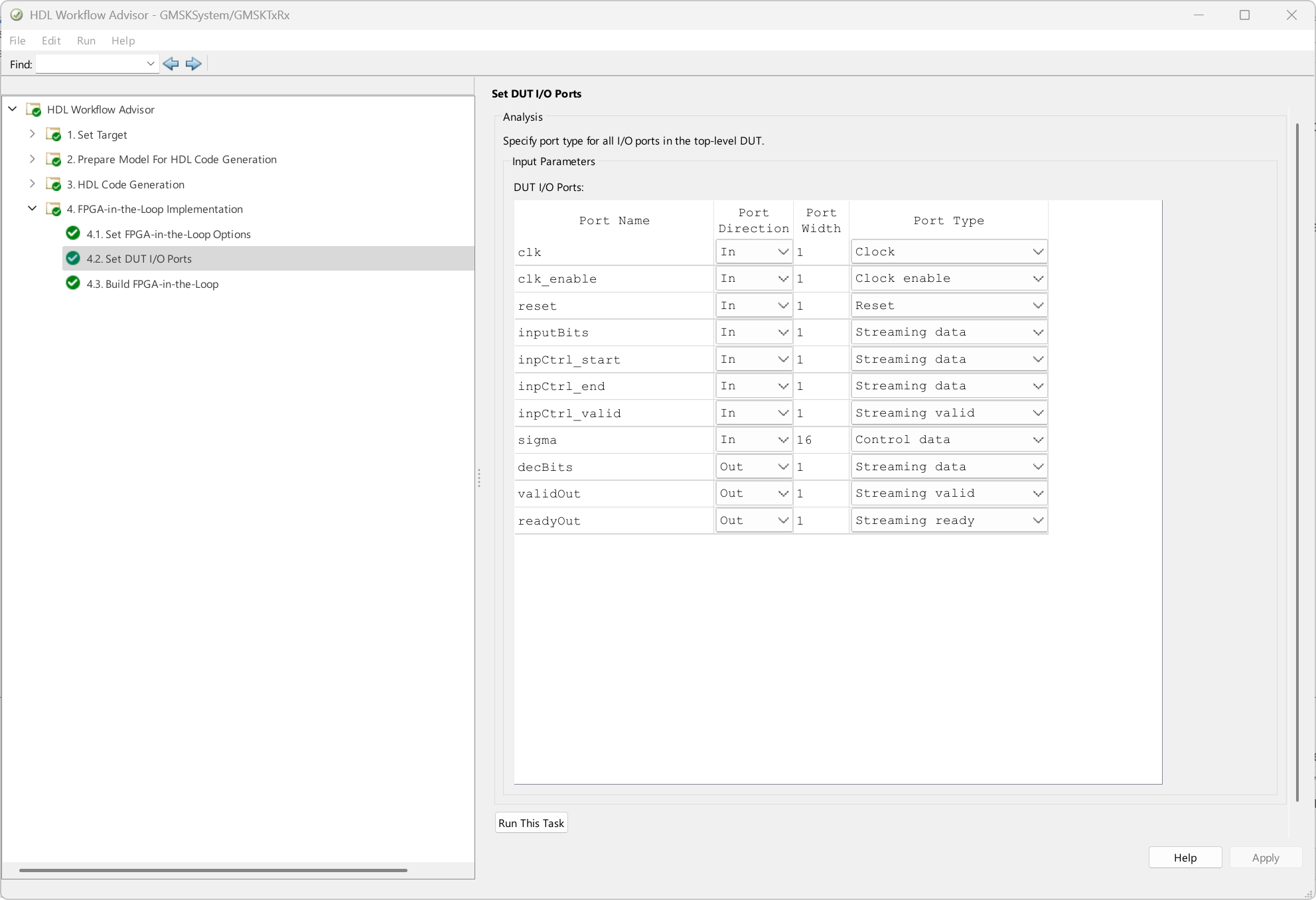
Under Set DUT I/O Ports, map the ports as the following figure shows. Because the value at the sigma port is constant for the duration of the inputBits, set its port type to Control data.

Complete the remaining steps to generate the Vivado project and MATLAB class files. A separate terminal window opens to complete synthesis and bitstream generation. This process also generates an interface script gs_GMSKTxRx_interface_fil.

The generated HDL code is synthesized for a ZCU102 Evaluation Kit. The post place and route resource utilization are shown in this table. The design meets the timing for a clock frequency of 200 MHz.

Resources	Usage
CLB LUT	9920
CLB Registers	7119
Block RAM Tile	7.5
DSPs	14

To run the simulation on the hardware, set the runBERonFPGA to true. Then, update the auto-generated interface script gs_GMSKTxRx_interface_fil to generate the BER curve for the chosen configuration, as shown in the following code. Use this code to send the inputs to the GMSK transmitter and receiver on the FPGA and read the decoded data back into MATLAB using the FIL free-running mode.

if runBERonFPGA
    filObj = GMSKTxRx_fil; %#ok<UNRCH>

    %% Program FPGA
    % If you need to change login parameters for your board, using the following syntax:
    % filObj.IPAddress = '192.168.0.2'; % modify to match the board IP address
    % filObj.Username = 'root';
    % filObj.Password = 'root';
    frameLen = 1e6;
    filObj.ReadFrameLength = frameLen;
    filObj.programFPGA;

    numFrames = 1000;
    EbNoVec = 0:10;
    SNRdB = convertSNR(EbNoVec,"ebno","snr",CodingRate=1/2,SamplesPerSymbol=2);
    noisePow  = 10.^(-SNRdB/10);
    sigma = sqrt(noisePow);
    BER_FPGA = zeros(length(EbNoVec),1);

    tic;
    for EbNoInd = 1:length(EbNoVec)
        bitErrors = 0;
        for frameCount = 1:numFrames
            % Generate random data and terminate for decoder
            actData = randn(frameLen,1)>0;
            actData(end-6:end) = 0;
            dataIn = actData;
            startIn = [true;false(frameLen-1,1)];
            endIn = [false(frameLen-1,1);true];

            % Write Control Data
            filObj.writePort('sigma', fi(sigma(EbNoInd),0,16,11));

            % Write Streaming Data
            filObj.writePort('inputBits', fi(dataIn,0,1,0),'inpCtrl_start', fi(startIn,0,1,0),'inpCtrl_end', fi(endIn,0,1,0));

            % Read Streaming Data
            [decBits]  = filObj.readPort('decBits');

            bitErrors = bitErrors + sum(xor(actData(1:length(decBits)),decBits));
        end
        BER_FPGA(EbNoInd) = bitErrors/numFrames/frameLen
    end
    toc;
    semilogy(EbNoVec,BER_FPGA,'r-*');
    grid on;
    title('BER on FPGA');
    xlabel('EbNo(dB)');
    ylabel('Bit Error Rate (BER)');

    %% Release hardware resources
    release(filObj);
end

Results

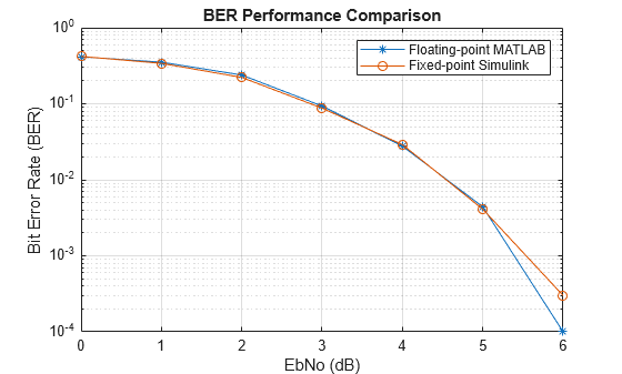
The example compares BER performance for floating-point and fixed-point implementations as shown in this figure.

figure;
semilogy(EbNoVec,BER_ML,'-*');
grid on;
hold on;
semilogy(EbNoVec,BER_SL,'-o');
xlabel('EbNo (dB)');
ylabel('Bit Error Rate (BER)');
legend('Floating-point MATLAB','Fixed-point Simulink');
title('BER Performance Comparison');
hold off;

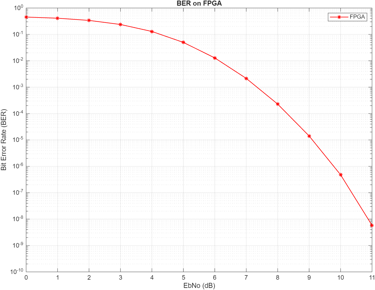
Running the BER simulations on the hardware is much faster even with a higher number of frames and a higher frame length. For a pulse length of 1 and samples per symbol of 2, the BER performance on the FPGA is shown below. This simulation uses a frame length of 1e7 and uses 1000 frames to generate this curve.

This example also shows execution time improvements when using FPGA acceleration. These results help demonstrate the tradeoffs between accuracy, resource usage, and speed. The following table summarizes the performance of the Simulink model and free-running FIL simulation modes. Free-running FIL significantly enhances simulation performance. It reduces simulation time to just 10 seconds, offering a remarkable 490 times improvement over the traditional Simulink behavioral model. This increase in speed is primarily due to the optimized data size in free-running mode, which outputs only valid data.

Simulation Mode	Time Taken (in seconds)	Performance Improvement
Simulink model	4900	1x
Free-running FIL	10	490x

Further Exploration

You can apply this floating‑point to fixed‑point workflow and run BER simulations on hardware for any communication system with different modulations such as phase shift keying (PSK), quadrature amplitude modulation (QAM) and observe the difference in the overall evaluation time.