Optimize an AUV’s Center of Mass | AUV Deep Dive, Part 3
From the series: AUV Deep Dive
Once you have your mechanism imported into Simulink®, you can run many kinds of optimizations, such as moving the center of mass of an underwater vehicle to maximize its restoring moment.
Published: 30 Apr 2021
So in the previous video, once we had the car parts brought in to the Simscape multi-body, we can apply hydrostatic forces. And to the point I was making about the restoring moment is how important it is for the buoyancy center and the center of mass of the vehicle to be very well aligned so that restoring moment acts in the right way.
So one of the big powerful things that we can do once we have that mechanism in Simscape multi-body, it's not just the fact we're bringing the mechanism, is that we are putting it in Simulink and Simulink lives on top of MATLAB, which has lots of very powerful control design capabilities and optimization capabilities.
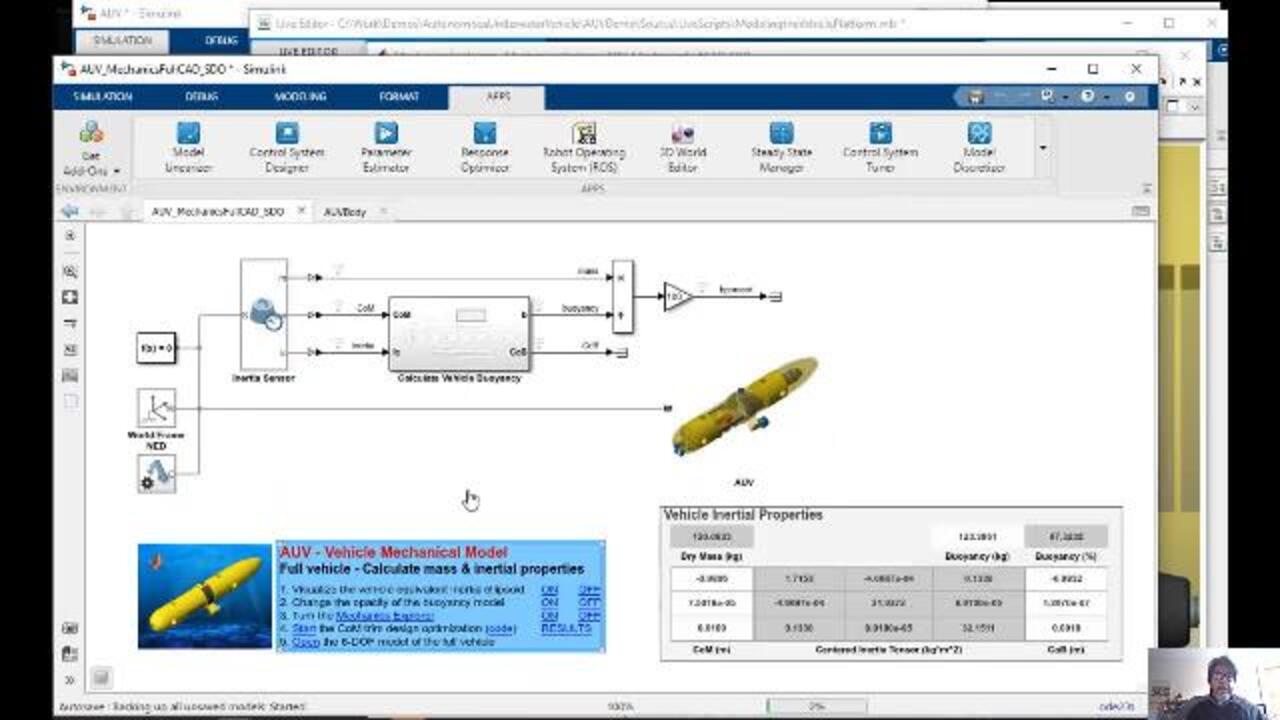
So for this example, what I am going to show is I have the car as we imported it from SolidWorks, so the center of mass and the center of buoyancy are very close to each other. So we could choose to live with this. But what I'm going to do is I'm going to run an optimization where I can play with the location of a couple of masses.
So if you look at my battery pack, I have a couple of transformers here that are locating an x direction for the trimming mass and the y direction for the trimming mass. So based on those two variables, I am trying to allocate my battery pack in a way where I can minimize the distance of these two frames.
In order to set up that optimization problem, I'm going to use a tool called Simulink Design Optimization. So if you go to the Apps tab in Simulink, we have a tool called a response optimizer. They allow you to hook up your Simulink model. Whatever your Simulink model is, allows you to allow you to hook it up to our optimization toolbox in MATLAB.
So you can set up any kind of requirements or characteristics in time domain, in frequency domain, you want to match a certain performance, a certain performance curve, a certain custom function in MATLAB. I have a little example script already set up.
So what this is going to do is it's going to allow that interface that I just showed you but is going to load it up with the project already set. What you're, seeing here is I have put a couple of constraints, a couple of constraints on the error. The x distance between the two frames and the y distance between the two frames.
What I'm setting my optimizer to do is to minimize that distance, to bring whatever the error in x and whatever the error in y is as close to zero, as we possibly can. This optimization problem is using the simulation model under the hood. So it's going to be running the simulation and recalculating.
At every simulation, is going to recalculate the new center of mass, the new center of buoyancy, and is going to be calculating the error between those two frames. So what you're seeing here is how it's changing the x location and the y location and how the error is coming. It was already pretty small. Again these are scaled values. So it doesn't mean 100 millimeters.
You can see the cost function for each one. It's going to run a number of simulations perturbing these variables. It perturbs in one direction, perturbs in the other direction and figures out, OK what gets me closer to the minimizing the cost function and keeps on going in that direction. Instead of manually
changing the numbers and guessing and guessing, this is using an actual optimization algorithm to perform this operation.
So you bring your mechanism and now I can perform a quick optimization problem on that mechanism. So we run a total of actually 63 simulations really to do the optimization. You can see how the values actually converge. So the optimization is finished and it has converged to the tolerances that I had specified and now all those variables are updated in the model.
So if I go back to the model and run the simulation again, what is going to happen is now we're going to see the new location of the center of mass and the center of buoyancy. So I don't know if you guys recall where we had at the beginning where it was a little off an x and a little off on y. Now pretty much below, exactly below if we look at it from the top.
You see like the top frame is completely obscuring the other frame really. So they're pretty much aligned to each other to whatever tolerance we have set on the optimisation. This is a geometric optimization. This optimization capability can be done for many, many other tasks.
So you may want to optimize the energy consumption for a particular maneuver, so then you can set up. As long as you set up the right requirements to, in this case, we can measure the amount of current that is being drawn from the models and optimize the time to do a maneuver or optimize the amount of power that is required for a maneuver.


