Differential Equations and Linear Algebra, 8.1c: Fourier Series Solution of Laplace's Equation
From the series: Differential Equations and Linear Algebra
Gilbert Strang, Massachusetts Institute of Technology (MIT)
Inside a circle, the solution u(r, θ) combines rn cos(nθ) and rn sin(nθ). The boundary solution combines all entries in a Fourier series to match the boundary conditions.
Published: 27 Jan 2016
OK. So this is using Fourier series. So I had to pick an equation where we were given a function, and not just a couple of initial values. So I made the equation a partial differential equation. The most famous one, Laplace's equation.
So this is the setup. And you'll see how Fourier series comes in. We're in a circle. I'm going to make this a nice model problem.
So inside this circle we're solving Laplace's equation. Laplace's equation was the second derivative of u in the x direction, plus the second derivative of u in the y direction, is 0. That's the way heat, temperature, distributes itself when you leave it alone.
In this problem I'm going to put a source of heat at that point. So it'll be a point source. A delta function. And on the rest of the boundary, temperature 0. So the boundary function is a delta function with a spike at that one point, and 0 elsewhere.
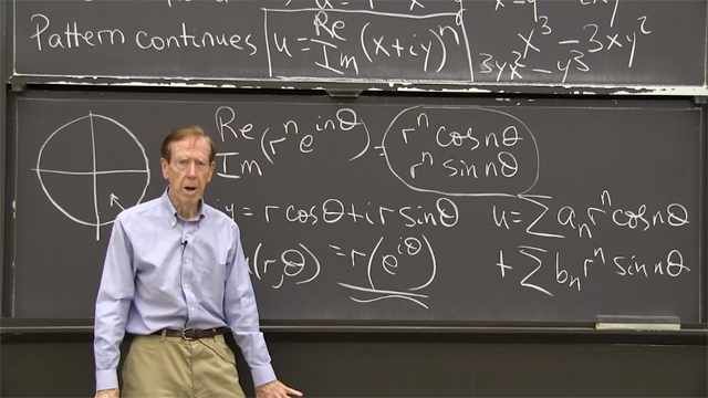
And our problem is to solve the Laplace's equation inside the circle. And we use polar coordinates because we've got a circle. So there is the equation with x and y, but we really are thinking r and theta. And the reason is, you get beautiful solutions to this equation using r and theta.
And that was a family of solutions. r to the n-th cos n theta just works. And so does r to the n-th sine n theta. And that's for every n.
So we have-- we can combine. We have a linear equation. We can take combinations of solutions with coefficients a n in the cosines, and bn in the sines.
And now here's the key step. Put in r equal 1. Put r equal 1. And then this solution, u at 1 and theta-- r equal 1-- is the boundary. It's the circle.
And that's where we're given u of 1 to be the delta function. The point source. The delta function. Delta of theta. The point source at theta equals 0.
So you see our job. That function, that boundary condition, is supposed to tell us the a's and the b's. And then we have our solution.
So by putting r equal to 1 in this formula, we're supposed to get the delta function. So let me put r equal 1. Easy to do. It's the sum of a n, 1 to the n-th, cos n theta, plus the sum of bn, 1 to the n-th, sine n theta, is supposed to match the delta function.
So that's the Fourier series for the delta function. That's the whole point. That we use a Fourier series expression for the boundary function, whatever that boundary function is. Here it's a particularly nice neat one.
And actually, the delta function is an even function. It's 0 at theta and it's 0 at minus theta. So changing theta to minus theta still leaves me the spike at 0. So because it's an even function, I won't see any signs. I won't see any odd functions. The sine theta.
And I have an easy time to find the coefficients a n of the cosines. Actually, we did that directly from the formula for the a n's. Let me just remember that formula. The formula was a0 was 1 over 2 pi times the average.
a0 is the average value of the temperature. And the temperature on the boundary is delta theta. And that integrates to 1, and we get the answer 1 over 2 pi. That's the average temperature.
Isn't that a little weird? The temperature 0 except at one point. At that point it's a delta function with the coefficient 1 outside it. And then we get 1 over 2 pi as the average.
The other a n's, the coefficients of the cosines, are 1 over pi, times the integral of our delta function, times cos n theta d theta. And the delta function, that point source, picks out that number at theta equals 0. And that number is 1. So I'm getting 1 over pi. So finally I now know the a's and b's.
When I put those in, that tells me the solution. The solution-- now I can put r back in the picture-- it's a sum. Well, let me take the a0 term. The a0 is 1 over 2 pi-- that's the constant, that's the average-- plus the sum of 1 over pi cos n theta, from n equals 1 to infinity.
And r to the n-th. Sorry. r to the n-th.
So you see what happens. When r is 1, we have the Fourier series for the delta function. That's the very exceptional function that's given on the boundary.
As soon as r is less than 1, these r to the n-th's get small, and we have a series that adds up to a reasonable sum. And we can actually-- it's possible to add up that series. It's possible to add up that series. It's a geometric series if you switch from cosines to exponentials. That's usually the good way to get good formulas.
And here, so you can add it up. And I think there's a 1 over 2 pi still there. And I think it's 1 minus r squared, over 1 plus r squared, minus 2r cos theta.
Let me just be sure I got that right. Yep, looks good. Looks good.
And we could check if it's good. Let's take theta equal 0. So if we take theta equal 0. Let me draw that circle again. Theta equal 0. We're coming out on that ray. And we're expecting to see infinity when we get there, at r equal 1.
So theta equal 0. So let me just put that. On the ray, theta equal 0.
This is what you should do. We have a formula for all r and theta, but let's look at some particular points to see what's happening.
So along that ray, where theta is 0, I have 1 over 2 pi, 1 minus r squared, over 1 plus r squared, minus 2r. Because cos theta is 1. And 1 plus r squared, minus 2r, is 1 minus r squared. Right? Because cos theta is 1 on this ray. Theta is 0. Cos theta is 1.
And now 1 minus r will factor out of this. And I think we get 1 plus r. And we still have a 1 minus r down below. I like that. You don't often, for partial differential equations, get some nice expression for the solution. So that's the solution.
And as r goes to 1, this solution blows up. Right. The temperature is infinite on the boundary, but the temperature is something reasonable inside.
And at r equals 0, I have 1 over 2 pi. Well, of course. It's the average value. Right at the center that temperature is going to be the average on the boundary.
That's a natural key property of Laplace's equation. It averages everything. Actually, if I take a little circle in anywhere, those temperature in the center of that circle would be the average of the temperatures around the little circle. For all the circles. It's just the Laplace's equation. Solving Laplace's equation averages everything.
And the result is that the temperature function sort of smoothes out as I come in. Around the boundary it's far from smooth. There's a big jolt at theta equals 0. But if I look on that circle, or that circle, or this circle, the temperature is a nice smooth function.
And it's never going to be above the maximum on the boundary. And it's never going to be below the minimum on the boundary. Everything's being averaged.
So that's, you see, a use of the Fourier series. For one particular function. I could do another function, but I don't think I will.
I could take the function that's 1 on the top of the circle and minus 1 on the bottom half of the circle. OK, that's a function with a jump, but not a delta function. So we would see a Fourier series that would give us the a's and the b's. There would probably only be b's in that case. Sine. Sine terms. And we'd get an answer.
May I just, while I'm talking about averages, add one final comment. Usually, for a complicated region, we can't solve Laplace's equation with formulas. It's not possible. We can't find sines and cosines that match some crazy boundary.
So we have to replace Laplace's equation. So I'll write Laplace's equation again. That goes into u-- we have a region. And we carve it out with a grid.
And then at each point on the grid, we have an equation connecting the value of u at that point. Say u0 at the center. With u east, maybe, u west, u north, and u south.
So we have an equation, and I want to write that equation down. u center is just going to be the average. It's just going to be 1/4 of u east, u west, u north, and u south.
So that'll be true at-- that equation will hold. The unknowns are all these u's. The u's of all the mesh points. And I have an equation at every mesh point.
So I have the same number of equations from the mesh points as unknowns at the mesh points. I solve that big system, and that gives me a solution u. An approximate solution u to Laplace's equation. So this would be called Laplace's difference equation, or Laplace's five-point scheme, because it uses five points in that average.
OK. That's an important problem in numerical analysis. Thank you.

