5G Beamforming with Ray Tracing Channels
This example shows how to calculate the beamforming weights for a 5G link in a ray tracing channel. The example uses two approaches to calculate the beamforming weights: singular value decomposition (SVD) and precoding matrix indicator (PMI) codebook search.
Introduction
Beamforming is a fundamental technique in 5G NR systems that improves link performance by directing energy toward the intended user. This example shows how to compute beamforming weights for a 5G link in a realistic ray tracing channel that models reflections and diffractions from buildings. The example uses two approaches to calculate the beamforming weights: SVD, which derives weights from the channel matrix, and PMI selection, which searches standardized codebooks defined in 3GPP TS 38.214 Section 5.2.2.2.
Configure Base Station and User Equipment
Specify the carrier frequency, subcarrier spacing, and the number of resource blocks.
fc = 4.2e9;   % Carrier frequency (Hz)
SCS = 15;     % Subcarrier spacing (kHz)
NRB = 52;     % Number of resource blocks
Specify the base station and user equipment (UE) locations.
bsPosition = [22.287495, 114.140706]; % lat, lon
uePosition = [22.287960, 114.141406]; % lat, lon
Configure the antenna arrays. Both the base station and the UE use rectangular arrays with the structure shown in the figure, where each position in the array contains two cross-polarized antenna elements. and are the number of columns and rows in the array, respectively.
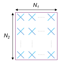
This example assumes the number of transmit or base station antennas is the same as the number of CSI-RS antenna ports. The set of valid base station array panel dimensions are specified in TS 38.214 Table 5.2.2.2.1-2.
Number of CSI-RS Antenna Ports | |
4 | (2, 1) |
8 | (2, 2) |
8 | (4, 1) |
12 | (3, 2) |
12 | (6, 1) |
16 | (4, 2) |
16 | (8, 1) |
24 | (4, 3) |
24 | (6, 2) |
24 | (12, 1) |
32 | (4, 4) |
32 | (8, 2) |
32 | (16, 1) |
N1 = 6;                       % Number of columns in panel
N2 = 2;                       % Number of rows in panel
bsArrayOrientation = [0; -6]; % Azimuth (0 deg is East, 90 deg is North) and elevation (positive points upwards) in deg
bsArraySize = [N2 N1];        % Base station panel dimensions [N2 N1] (rows, columns)
validatePanelDimensions(flip(bsArraySize))
Specify the UE array size and the UE orientation in azimuth and elevation.
ueArraySize = [2 2];            % Number of rows and columns in rectangular array (UE)
ueArrayOrientation = [180; 45]; % Azimuth (0 deg is East, 90 deg is North) and elevation (positive points upwards) in deg
Specify the maximum number of reflections and diffractions for ray tracing.
numReflections = 2;             % Number of reflections for ray tracing analysis (0 for LOS)
numDiffractions = 1;            % Number of diffractions for ray tracing analysis
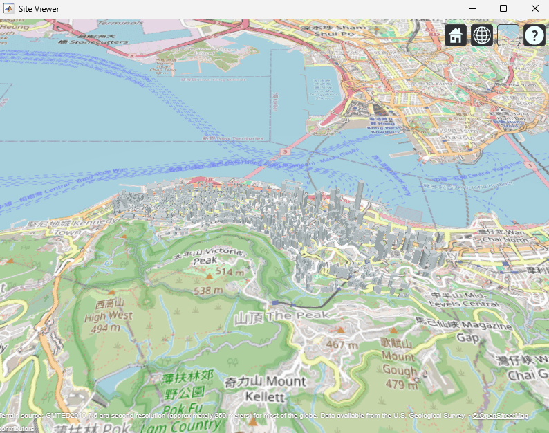
Import and Visualize 3-D Environment with Buildings for Ray Tracing
Open Site Viewer with buildings in Hong Kong [1].
if exist("viewer","var") && isvalid(viewer) % Viewer handle exists and viewer window is open
    clearMap(viewer);
else
    viewer = siteviewer("Basemap","openstreetmap","Buildings","hongkong.osm");
end
Create Base Station and UE Sites
Place the base station and UE objects on the map. These objects are the means for ray tracing.
Create a single-panel base station array with antenna elements defined in TS 38.901.
lambda = physconst("LightSpeed")/fc;
bsArray = phased.NRRectangularPanelArray(Size=[bsArraySize 1 1],Spacing=[0.5*lambda*[1 1] 1 1]);
bsArray.ElementSet = {phased.NRAntennaElement(PolarizationAngle=45),phased.NRAntennaElement(PolarizationAngle=-45)};
Create the base station object.
bsSite = txsite(Name="Base station", ...
    Latitude=bsPosition(1),Longitude=bsPosition(2), ...
    Antenna=bsArray, ...
    AntennaAngle=bsArrayOrientation, ...
    AntennaHeight=10, ...  % in m
    TransmitterFrequency=fc);
Create the UE array. Use short dipole antenna elements with cross polarization.
ueAnt1PolAngle = 0;                                         % First polarization angle in degrees
ueAnt2PolAngle = 90;                                        % Second polarization angle in degrees
pol1AntElement = createUEAntennaElement(ueAnt1PolAngle,fc); % Antenna element with first polarization angle
pol2AntElement = createUEAntennaElement(ueAnt2PolAngle,fc); % Antenna element with second polarization angle
ueArray = phased.NRRectangularPanelArray(Size=[ueArraySize 1 1],Spacing=[0.5*lambda*[1 1] 1 1]);
ueArray.ElementSet = {pol1AntElement, pol2AntElement};
Create the UE object.
ueSite = rxsite(Name="UE", ...
    Latitude=uePosition(1),Longitude=uePosition(2), ...
    Antenna=ueArray, ...
    AntennaAngle=ueArrayOrientation, ...
    AntennaHeight=1.5);
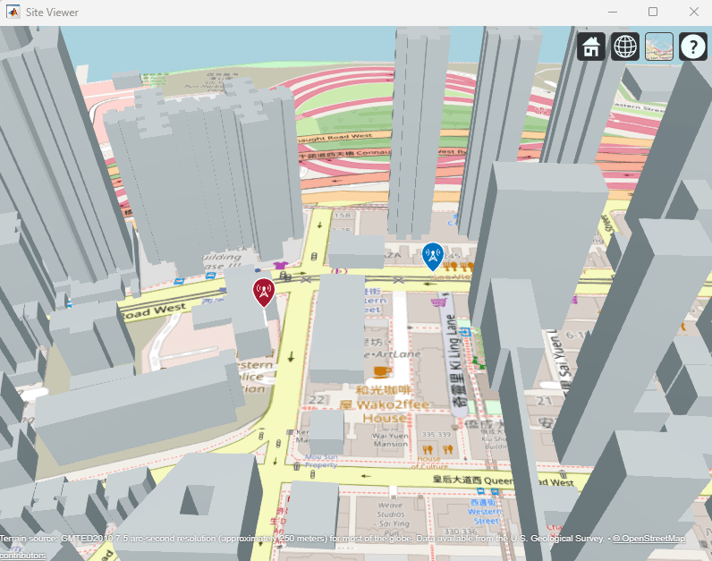
Visualize the location of the base station and the UE.
show(bsSite);
show(ueSite);
Perform Ray Tracing Analysis
Create a propagation model to perform ray tracing.
pm = propagationModel("raytracing",Method="sbr",MaxNumReflections=numReflections,MaxNumDiffractions=numDiffractions);
rays = raytrace(bsSite,ueSite,pm,Type="pathloss");
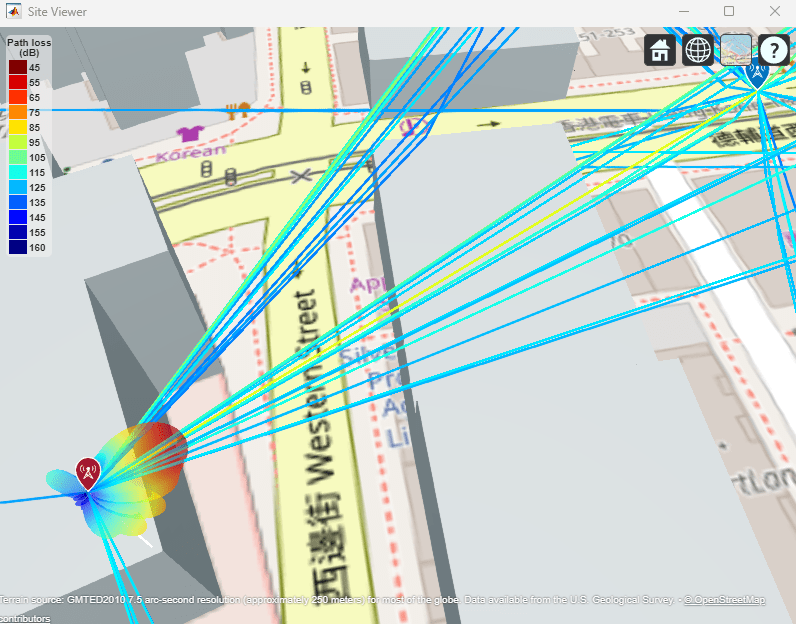
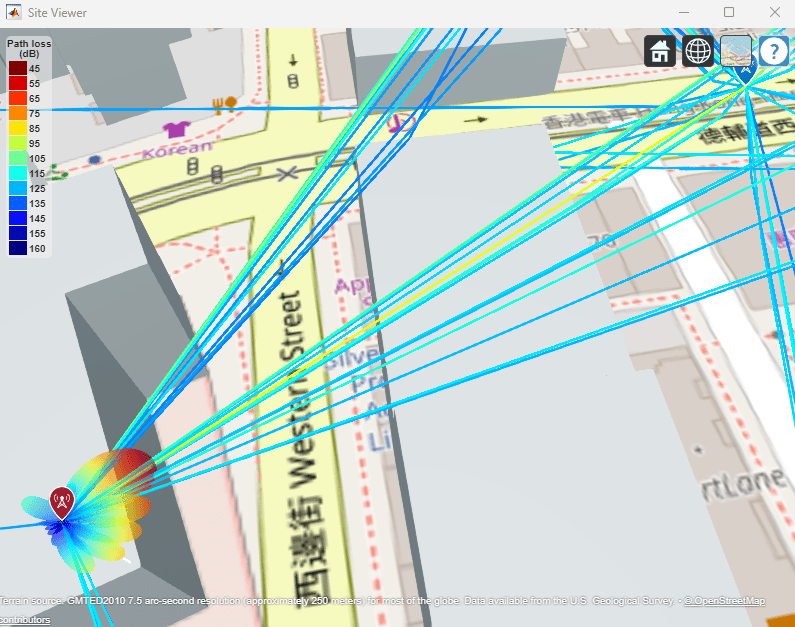
Display the rays in Site Viewer.
plot(rays{1})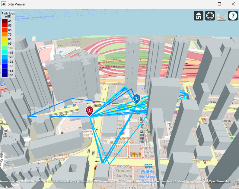
Create Ray Tracing Channel
Get OFDM-related information, including the sampling rate for the provided NRB and SCS values.
ofdmInfo = nrOFDMInfo(NRB,SCS);
Create a tracing channel model from the returned rays, the base station, and UE sites.
ch = comm.RayTracingChannel(rays{1},bsSite,ueSite);
ch.SampleRate = ofdmInfo.SampleRate;
ch.MinimizePropagationDelay = true;
Disable channel filtering. You can obtain the channel impulse response directly from the ray tracing channel, without filtering a signal.
ch.ChannelFiltering = false;
Because the ray tracing channel models a static scenario, to generate a single snapshot of the channel impulse response at a time, set ReceiverVirtualVelocity to 0 and NumSamples to 1.
ch.ReceiverVirtualVelocity = [0;0;0];
ch.NumSamples = 1; % 1 channel snapshot per channel call
The channel models the effect of path loss. Therefore, set NormalizeImpulseResponses to false. To stop the channel normalizing the impulse response by the number of receive antennas, set NormalizeChannelOutputs to false .
ch.NormalizeImpulseResponses = false;
ch.NormalizeChannelOutputs = false;
Calculate OFDM Channel Response of Ray Tracing Channel
Get the channel impulse response.
cir = ch();
Calculate the OFDM channel response.
% Get channel filter coefficients
chInfo = ch.info();
pathFilters = chInfo.ChannelFilterCoefficients;
% Carrier object used to get OFDM channel response
carrier = nrCarrierConfig(SubcarrierSpacing=SCS,NSizeGrid=NRB);
% OFDM channel response
hest = nrPerfectChannelEstimate(carrier,cir,pathFilters.');
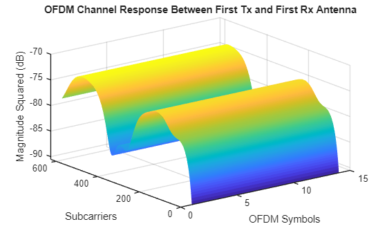
Plot the OFDM channel response in time and frequency between the first transmit and the first receive antenna. This plot shows how the channel behaves in frequency (subcarriers) and time during the observation period of one slot.
surf(pow2db(abs(hest(:,:,1,1)).^2));
shading("flat");
xlabel("OFDM Symbols");ylabel("Subcarriers");zlabel("Magnitude Squared (dB)");
title("OFDM Channel Response Between First Tx and First Rx Antenna");
Get Beamforming Weights Using SVD
Calculate the beamforming weights using SVD. Assume one layer. The getBeamformingWeights function averages the channel conditions over a number of resource blocks, starting at an offset from the edge of the band (first subcarrier), and enables subband beamforming.
nLayers = 1;
scOffset = 0;   % No offset
noRBs = 1;      % Average channel conditions over 1 RB to calculate beamforming weights
wbsSVD = getBeamformingWeights(hest,nLayers,scOffset,noRBs);
Plot the base station radiation pattern associated with the beamforming weights obtained using SVD.
bsSite.Antenna = clone(ch.TransmitArray); % Need a clone, otherwise setting the Taper weights affects the channel array
bsSite.Antenna.Taper = wbsSVD;
pattern(bsSite,fc,"Size",5);
Get Beamforming Weights Using PMI Selection
Calculate the beamforming weights using the PMI selection process. The code iterates over all precoding matrices in the type I single panel codebook (TS 38.214 Tables 5.2.2.2.1-1 to 5.2.2.2.1-12) and selects the precoding matrix that maximizes the SINR for a given channel matrix and noise variance.
Construct the CSI reporting structure and the CSI-RS configuration. The code selects a valid CSI-RS configuration.
reportConfig = struct();
reportConfig.NSizeBWP = [];
reportConfig.NStartBWP = [];
reportConfig.CodebookType = "type1SinglePanel";
reportConfig.PanelDimensions = [N1 N2];

% Get a valid CSI-RS configuration
[rowNumber,numSubcarrierLocations,numSymbolLocations] = getCSIRSRow(2*prod(bsArraySize));
csirs = nrCSIRSConfig;
csirs.NumRB = NRB;
csirs.RowNumber = rowNumber;
csirs.SubcarrierLocations = (1:numSubcarrierLocations)-1;
csirs.SymbolLocations = 2*((1:numSymbolLocations)-1);
The PMIInfo structure contains the precoding matrix indicator and the beamforming weights.
[PMISet,PMIInfo] = hDLPMISelect(carrier,csirs,reportConfig,nLayers,hest);
Plot the base station radiation pattern associated with the PMI beamforming weights.
bsSite.Antenna = clone(ch.TransmitArray); % Need a clone, otherwise setting the Taper weights affects the channel array
bsSite.Antenna.Taper = PMIInfo.W;
pattern(bsSite,fc,"Size",5);
References
[1] The example uses an OSM file downloaded from https://www.openstreetmap.org, which provides access to crowd-sourced map data all over the world. The data is licensed under the Open Data Commons Open Database License (ODbL), https://opendatacommons.org/licenses/odbl/.
Local Functions
function [wtx,wrx,D] = getBeamformingWeights(hEst,nLayers,scOffset,noRBs)
    % Get beamforming weights given a channel matrix hEst and the number of
    % layers nLayers. One set of weights is provided for the whole
    % bandwidth. The beamforming weights are calculated using singular
    % value decomposition (SVD).
    %
    % Only part of the channel estimate is used to get the weights, this is
    % indicated by an offset SCOFFSET (offset from the first subcarrier) and a
    % width in RBs (NORBS).

    % Average channel estimate
    [~,~,R,P] = size(hEst);
    scNo = scOffset+1;
    hEst = hEst(scNo:scNo+(12*noRBs-1),:,:,:);
    H = permute(mean(reshape(hEst,[],R,P)),[2 3 1]);

    % SVD decomposition
    [U,D,V] = svd(H);
    wtx = V(:,1:nLayers).';
    wrx = U(:,1:nLayers)';
end

function ueAntennaElement = createUEAntennaElement(polAngleDeg,fc)
    % Create a custom antenna element using a short dipole element as a
    % reference. POLANGLEDEG is the polarization angle in degrees relative to
    % the z axes of the reference short dipole element. FC is the frequency
    % used to calculate the antenna response.

    % Compute polarization direction vector
    polVector = [0; sind(polAngleDeg); cosd(polAngleDeg)]; % y–z plane rotation

    % Create reference short dipole antenna element
    shortDipole = phased.ShortDipoleAntennaElement(AxisDirection='Custom',CustomAxisDirection=polVector);

    % Define angles
    azAngles = -180:180;  % Azimuth angles
    elAngles = -90:90;    % Elevation angles

    % Extract H and V patterns in magnitude and phase
    patHmag = zeros(numel(elAngles),numel(azAngles));
    patVmag = patHmag;
    patHphase = patHmag;
    patVphase = patHmag;

    for m = 1:numel(elAngles)
        pat = step(shortDipole,fc,[azAngles;elAngles(m)*ones(1,numel(azAngles))]);

        patHmag(m,:) = mag2db(abs(pat.H));      % Store horizontal pattern magnitude
        patVmag(m,:) = mag2db(abs(pat.V));      % Store vertical pattern magnitude
        patHphase(m,:) = rad2deg(angle(pat.H)); % Store horizontal pattern phase
        patVphase(m,:) = rad2deg(angle(pat.V)); % Store vertical pattern phase
    end

    % Initialize the custom antenna element with polarization applied
    ueAntennaElement = phased.CustomAntennaElement(PatternCoordinateSystem='az-el', ...
                    AzimuthAngles=azAngles,ElevationAngles=elAngles, ...
                    SpecifyPolarizationPattern=true, ...
                    HorizontalMagnitudePattern=patHmag,HorizontalPhasePattern=patHphase, ...
                    VerticalMagnitudePattern=patVmag,VerticalPhasePattern=patVphase);
end

function validatePanelDimensions(panelDimensions)
% Validate panelDimensions against valid values from
% TS 38.214 Table 5.2.2.2.1-2
%
% Valid values:
% (2,1), (2,2), (4,1), (3,2), (6,1), (4,2), (8,1),
% (4,3), (6,2), (12,1), (4,4), (8,2), (16,1)

    % Define valid panel dimensions (N1, N2)
    validDims = [2 1;
                 2 2;
                 4 1;
                 3 2;
                 6 1;
                 4 2;
                 8 1;
                 4 3;
                 6 2;
                 12 1;
                 4 4;
                 8 2;
                 16 1];

    % Check if panelDimensions matches any valid pair
    if ~ismember(panelDimensions(:).', validDims, "rows")
        error("Invalid panelDimensions (N1, N2). Valid values are: "+ ...
            mat2str(validDims));
    end
end


function [rowNumber,numSubcarrierLocations,numSymbolLocations] = getCSIRSRow(numPorts)
% Mapping of Row to ports, number of subcarrier locations, and number
% of symbol locations from TS 38.211 Table 7.4.1.5.3-1
    rowPortsMap = [ 1 1 1 1;
                    2 1 1 1;
                    3 2 1 1;
                    4 4 1 1;
                    5 4 1 1;
                    6 8 4 1;
                    7 8 2 1;
                    8 8 2 1;
                    9 12 6 1;
                    10 12 3 1;
                    11 16 4 1;
                    12 16 4 1;
                    13 24 3 2;
                    14 24 3 2;
                    15 24 3 1;
                    16 32 4 2;
                    17 32 4 2;
                    18 32 4 1];

    % Find first rows numPorts
    rowIdx = find(rowPortsMap(:,2) == numPorts,1);

    if isempty(rowIdx)
        error("No row supports %d ports.", numPorts);
    else
        rowNumber = rowPortsMap(rowIdx,1);
        numSubcarrierLocations = rowPortsMap(rowIdx,3);
        numSymbolLocations = rowPortsMap(rowIdx,4);
    end
end
See Also
Functions
Objects
comm.RayTracingChannel|phased.NRRectangularPanelArray(Phased Array System Toolbox)