Verify Performance of 6G AI-Native Receiver Using MATLAB and PyTorch Coexecution
This example shows how to test a PyTorch® artificial intelligence (AI)-native receiver network and compare it to a conventional 5G receiver. The example demonstrates multi-process execution on central processing units (CPUs) and graphics processing units (GPUs).
Generate a data stream in MATLAB® and perform inference by using the PyTorch® network in an online data generation workflow. This approach enables inference with deep learning (DL) models without saving the data to disk.
To validate the PyTorch network, follow these steps:
Set up the Python® environment and verify required packages.
Specify test simulation parameters.
Load the PyTorch network.
Validate the network by using online data generation and testing.
Visualize and compare the results with a conventional 5G receiver benchmark.
System Description
This example provides a testbench for AI-native convolutional receivers also known as DeepRx [1]. The testbench supports online data generation, inference, and hardware acceleration. The fully convolutional DeepRx replaces 5G receiver operations with convolutional neural networks (CNNs) to improve performance under severe channel impairments and sparse pilot configurations. Under these conditions, traditional minimum mean squared error (MMSE)-based 5G receivers perform poorly, and DeepRx outperforms 5G receivers. For more information about AI-native receivers and implementation details, see the AI-Native Fully Convolutional Receiver example.
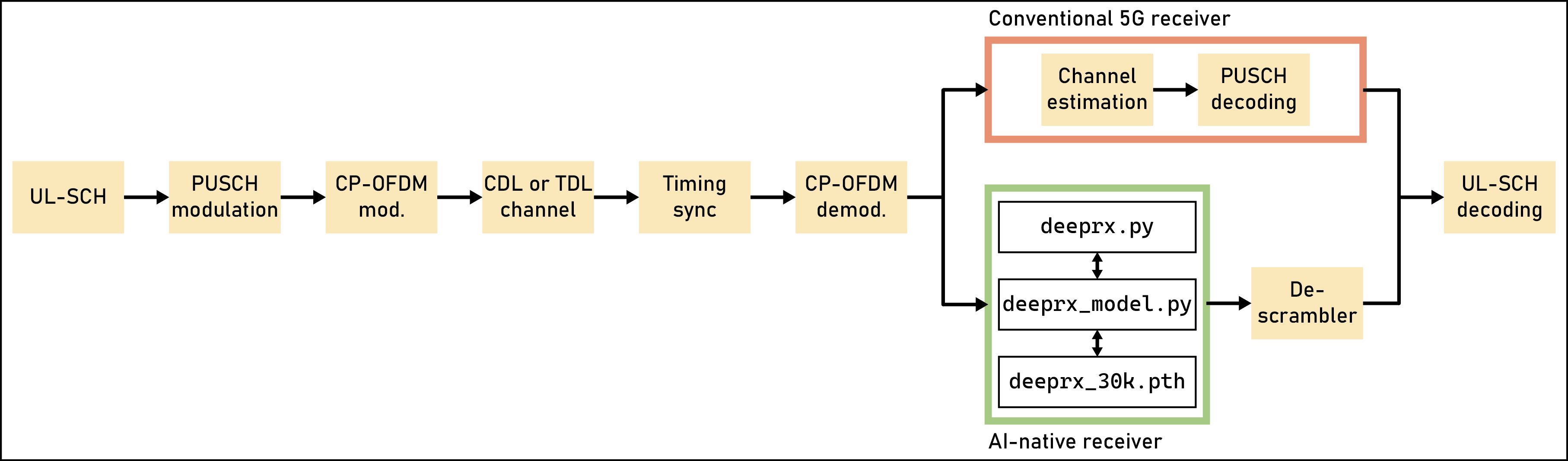
The following figure shows the physical uplink shared channel (PUSCH) simulation. The simulation measures coded bit error rate (BER) and throughput by using an AI-native convolutional receiver and compares the results with a conventional 5G receiver benchmark.
The
deeprx.pyscript contains PyTorch code that loads the model by usingdeeprx_model.pyanddeeprx_30k.pth, and performs log-likelihood ratio (LLR) predictions. These predictions replace channel estimation, channel equalization, and symbol demodulation in the conventional 5G receiver.The
deeprx_model.pyscript implements the MATLAB–Python interface and provides a common API for model construction (by usingdeeprx_30k.pth), data conversion, and prediction.The
deeprx_30k.pthfile stores the model state dictionary, including the model parameters (weights and biases) and optimizer states.
Step 1: Set Up Python Environment
Configure the Python environment to run the trained PyTorch network.
Before running this example:
Set up the Python environment as described in Call Python from MATLAB for Wireless.
Specify the full or relative path to the Python executable. The path can also point to a virtual environment.
On Windows®, specify the path to the
pythonw.exefile.
This example uses the OutOfProcess execution mode of the Python interpreter. If you use InProcess mode, MATLAB® and PyTorch might have library conflicts. For details, see pyenv.
% Configure the Python environment simParameters.PythonExecutionMode ="OutOfProcess"; % Paths for the Python executable: % ..\venv\Scripts\pythonw.exe for Windows and ../venv/bin/python3 for Linux simParameters.PythonPath = "relative_path_to_python_executable"; % Path to the REQUIREMENTS.txt file simParameters.PythonRequirements = "requirements_6GVerify.txt";
The helperSetupPyenv function configures the Python environment in MATLAB and verifies that the libraries listed in requirements_6GVerify.txt are installed.
currentPyEnv = helperSetupPyenv(...
    simParameters.PythonPath,...
    simParameters.PythonExecutionMode,...
    simParameters.PythonRequirements);
Setting up Python environment
Parsing requirements_6GVerify.txt
Checking required package 'torch'
Checking required package 'numpy'
Required Python libraries are installed.
Step 2: Specify Test Parameters
To test the performance of the AI-native receiver network:
Define the carrier, uplink shared channel (UL-SCH), PUSCH, and PUSCH demodulation reference signal (DM-RS) configurations, along with the channel parameters.
Select the propagation channels to validate the model. The example supports clustered delay line (CDL) and tapped delay line (TDL) channels.
This example calculates and compares the performance of the trained network with that of a conventional 5G receiver. The signal-to-noise ratio (SNR) parameter represents the SNR per resource element (RE) and per antenna element. For details, see the SNR Definition Used in Link Simulations example. To reduce execution time, run each SNR point on a separate worker. To enable CPU-based hardware acceleration for the end-to-end PUSCH simulation during test data generation, set simParameters.UseParallel to true. This option requires Parallel Computing Toolbox™.
% End-to-end simulation parameters for testing the AI-native and % conventional 5G receivers simParameters.UseParallel =false; % If true, enable parallel processing; otherwise, execute serially simParameters.ChannelModel =
"TDL-E"; % Channel models for testing: "CDL-A", "CDL-E", "TDL-A", "TDL-E" simParameters.DelaySpread =
100e-9; % Delay spread in seconds, range: [10e-9, 300e-9] simParameters.MaximumDopplerShift =
250; % Maximum Doppler shift in Hz, range: [0, 500] simParameters.SNRInVec =
0:10; % SNR range in dB for evaluation simParameters.ModulationType =
"QPSK"; % Modulation type: "QPSK" or "16QAM" simParameters.DMRSAdditionalPosition =
0; % DMRS additional position: 0 or 1 simParameters.DMRSConfigurationType =
2; % DMRS configuration type: 1 or 2 simParameters.NFrames =
5; % Number of frames for the simulation simParameters.PerfectChannelEstimator =
false; % Use perfect channel estimation if true % Generic UL PUSCH simulation parameters comes from [1] simParameters.CarrierFrequency = 3.5e9; % Carrier frequency in Hz simParameters.NSizeGrid = 26; % Number of resource blocks (26 RBs at 15 kHz SCS) simParameters.SubcarrierSpacing = 15; % Subcarrier spacing in kHz simParameters.CodeRate = 658/1024; % Code rate used to calculate transport block size % Additional UL PUSCH simulation parameters simParameters = hConfigureSimulationParameters(simParameters); % AI/ML parameters simParameters = configureAIMLParameters(simParameters); % Display the simulation parameter summary displayParameterSummary(simParameters);
________________________________________

Simulation Summary
________________________________________

- Input (X) size:                   [ 312   14   10 ]
- Output (L) size:                  [ 312   14    2 ]

- Number of subcarriers (F):        312
- Number of symbols (S):            14
- Number of receive antennas (Nrx): 2
Step 3: Load PyTorch Network
To load the PyTorch network into the example workspace and inspect its properties:
Locate the model file by using the
simParameters.ModelPathparameter.Create a PyTorch model instance by using the
hCreateTorchDeepRxfunction and load the trained network parameters.Display the model details.
Locate the model parameter file in
.pthformat in the example workspace for validation. By default, this example stores the parameter dictionary in a.zipfile, which thehCreateTorchDeepRxfunction unzips.
simParameters.ModelPath   = "deeprx_30k.pth";
simParameters.ModelInput  = simParameters.InputSize;
simParameters.ModelOutput = [simParameters.ModelInput(1:2) 4];
Create the PyTorch DeepRx network instance in MATLAB by calling hCreateTorchDeepRx and specifying the input and output sizes, and , respectively.
— Total number of subcarriers.
— Total number of OFDM symbols in the input resource grid.
— Number of input channels. The grid stacks
rxGrid,dmrsGrid, andrawChanEstGrid, where .— Number of receive antennas.
— Number of bits per transmitted symbol (e.g., 2 for QPSK, 4 for 16-QAM).
This example fixes the model input and output sizes as and because it uses the same training parameters as the AI-Native Fully Convolutional Receiver example. For architecture details, see Details of AI-Native Fully Convolutional Receiver Network.
After you load the network, you can test QPSK or 16-QAM. The bit-masking logic supports constellations with modulation order less than or equal to the training modulation order [1].
By default, the
hCreateTorchDeepRxfunction instantiates the model in evaluation mode. The function usesdeeprx_30k.pthto load the trained model and optimizer parameters. In evaluation mode, the batch normalization layers in the DeepRx architecture use the stored running mean and variance instead of the current batch statistics.To instantiate an untrained model without loading pretrained parameters, set
simParameters.ModelPathtostring.emptyor[].
model = hCreateTorchDeepRx(simParameters);
Display the network summary to view the model details.
modelParameters = py.deeprx.info(model);
displayNetworkSummary(modelParameters);
________________________________________

Neural Network Summary
________________________________________

- Total number of learnables: 1.2325 million
- Number of layers          : 13

- Model building blocks     :
			      1) conv_in
			      2) resnet_block_1
			      3) resnet_block_2
			      4) resnet_block_3
			      5) resnet_block_4
			      6) resnet_block_5
			      7) resnet_block_6
			      8) resnet_block_7
			      9) resnet_block_8
			     10) resnet_block_9
			     11) resnet_block_10
			     12) resnet_block_11
			     13) conv_out
Step 4: Test and Compare AI-Native Receiver Against Benchmark
In this section, you:
Generate a batch of test data.
Make predictions by using the AI-native PyTorch receiver network and a conventional 5G receiver.
Calculate and compare the coded BER and throughput.
The evaluateLinkPerformance function evaluates the AI-native and conventional 5G receivers based on the simulation parameters from Step 2.
If
simParameters.UseParallelistrue, the example creates aparforloop and schedules thehEvaluatePUSCHAtSNRfunction to run on each worker. Each worker processes one SNR point (simParameters.SNRIn). When executed on a worker, thehEvaluatePUSCHAtSNRfunction sets up the Python environment (pyenv) and loads the model.
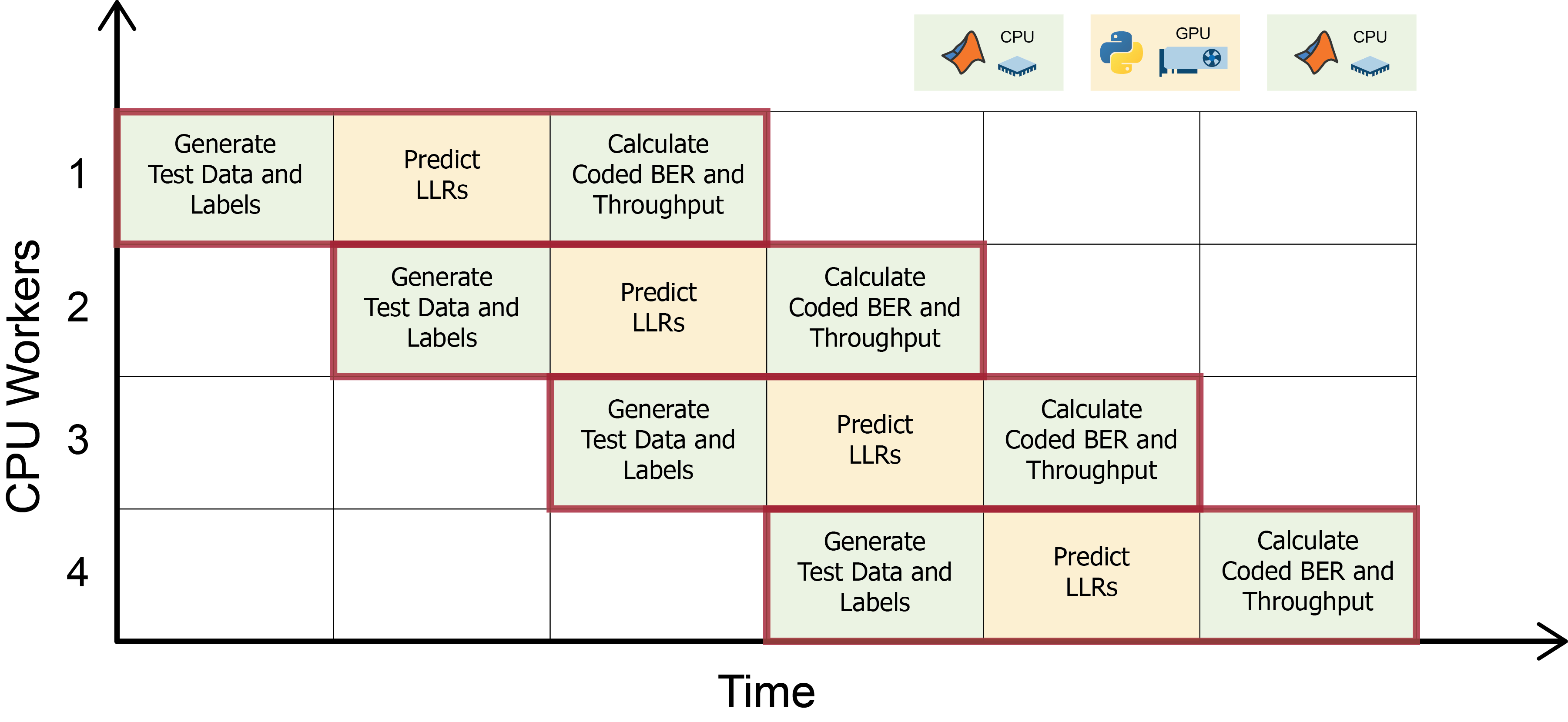
Otherwise, the number of workers in the
parforloop is set to0. In this case, each SNR point (simParameters.SNRIn) runs sequentially on a single CPU process. The simulation calculates the coded bit error rate (BER) and throughput for the AI-native and conventional 5G receivers.
This example uses CUDA®-based GPU acceleration in PyTorch (if available) by sending the model to the GPU in Step 3. Similarly, the predict function in the deeprx module sends the test data tensors to the GPU for accelerated prediction.
To simulate the end-to-end 5G New Radio (NR) link link, call the hCreateTorchDeepRx function inside the hEvaluatePUSCHAtSNR function. The following code snippets show how the AI-native and conventional 5G receivers determine the LLR values inside hEvaluatePUSCHAtSNR by using the default example parameters.
This code shows the LLR prediction and
ulschLLRscalculation when the AI-native receiver model is passed to thehRecoverPUSCHTorchDeepRxfunction.
% Predict LLRs using the input resource grids
L = single(py.deeprx.predict(net, X));

% Extract utilized LLRs. Note that the negation comes from the
% difference between the LLR definition in `ldpcDecode` and BCE loss
% functions.
Qm = puschIndicesInfo.G / puschIndicesInfo.Gd / pusch.NumLayers;
extractedLLRs = nrExtractResources(double(puschIndices), -L(:, :, 1:Qm));
ulschLLRs = reshape(gather(extractedLLRs.'), [], 1);
ulschLLRs = nrPUSCHDescramble(ulschLLRs, simLocal.PUSCH.NID, simLocal.PUSCH.RNTI, []);
Similarly, this code shows the
ulschLLRscalculation for practical channel estimation when the conventional 5G receiver is used in thehRecoverPUSCHConventionalfunction.
% Practical channel estimation between the received grid and each
% transmission layer, using the PUSCH DM-RS for each layer which
% are created by specifying the non-codebook transmission scheme
dmrsLayerSymbols = nrPUSCHDMRS(carrier, puschNonCodebook);
dmrsLayerIndices = nrPUSCHDMRSIndices(carrier, puschNonCodebook);
[estChannelGrid,noiseEst] = nrChannelEstimate(carrier, rxGrid, dmrsLayerIndices, dmrsLayerSymbols, 'CDMLengths', pusch.DMRS.CDMLengths);

% Extract PUSCH resource elements from the received grid
[puschRx, puschHest] = nrExtractResources(puschIndices, rxGrid, estChannelGrid);

% Equalization using MMSE
[puschEq,csi] = nrEqualizeMMSE(puschRx, puschHest, noiseEst);

% Decode PUSCH physical channel
[ulschLLRs, rxSymbols] = nrPUSCHDecode(carrier, puschNonCodebook, puschEq, noiseEst);
% Link performance evaluation; results will return coded BER and throughput
[resultsRX, resultsAI] = compareReceiverPerformance(simParameters);
________________________________________ Simulating DeepRx and 5G receivers ________________________________________ - Test data generation: Serial execution - Inference environment: CUDA Simulating DeepRx and conventional receivers for 11 SNR points... SNRIn: +10.00 dB | Channel: TDL-E | Delay spread: 1.00e-07 | Max Doppler shift: 250.00 | DMRS Add. Pos. / Config. Type: 0 / 2 SNRIn: +9.00 dB | Channel: TDL-E | Delay spread: 1.00e-07 | Max Doppler shift: 250.00 | DMRS Add. Pos. / Config. Type: 0 / 2 SNRIn: +8.00 dB | Channel: TDL-E | Delay spread: 1.00e-07 | Max Doppler shift: 250.00 | DMRS Add. Pos. / Config. Type: 0 / 2 SNRIn: +7.00 dB | Channel: TDL-E | Delay spread: 1.00e-07 | Max Doppler shift: 250.00 | DMRS Add. Pos. / Config. Type: 0 / 2 SNRIn: +6.00 dB | Channel: TDL-E | Delay spread: 1.00e-07 | Max Doppler shift: 250.00 | DMRS Add. Pos. / Config. Type: 0 / 2 SNRIn: +5.00 dB | Channel: TDL-E | Delay spread: 1.00e-07 | Max Doppler shift: 250.00 | DMRS Add. Pos. / Config. Type: 0 / 2 SNRIn: +4.00 dB | Channel: TDL-E | Delay spread: 1.00e-07 | Max Doppler shift: 250.00 | DMRS Add. Pos. / Config. Type: 0 / 2 SNRIn: +3.00 dB | Channel: TDL-E | Delay spread: 1.00e-07 | Max Doppler shift: 250.00 | DMRS Add. Pos. / Config. Type: 0 / 2 SNRIn: +2.00 dB | Channel: TDL-E | Delay spread: 1.00e-07 | Max Doppler shift: 250.00 | DMRS Add. Pos. / Config. Type: 0 / 2 SNRIn: +1.00 dB | Channel: TDL-E | Delay spread: 1.00e-07 | Max Doppler shift: 250.00 | DMRS Add. Pos. / Config. Type: 0 / 2 SNRIn: +0.00 dB | Channel: TDL-E | Delay spread: 1.00e-07 | Max Doppler shift: 250.00 | DMRS Add. Pos. / Config. Type: 0 / 2
Step 5: Visualize Results
Use the visualizePerformance local function to plot the coded BER and throughput of the AI-native and conventional 5G receivers across the SNR range. The resulting figures show that the AI-native receiver significantly outperforms the conventional receiver for the given scenario parameters.
% Plot Coded BER vs. SNR and Throughput (%) vs. SNR
visualizePerformance(simParameters,resultsRX,resultsAI);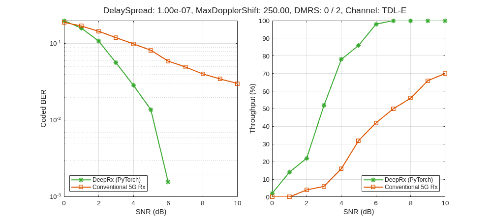
Further Exploration: Details of AI-Native Fully Convolutional Receiver Network
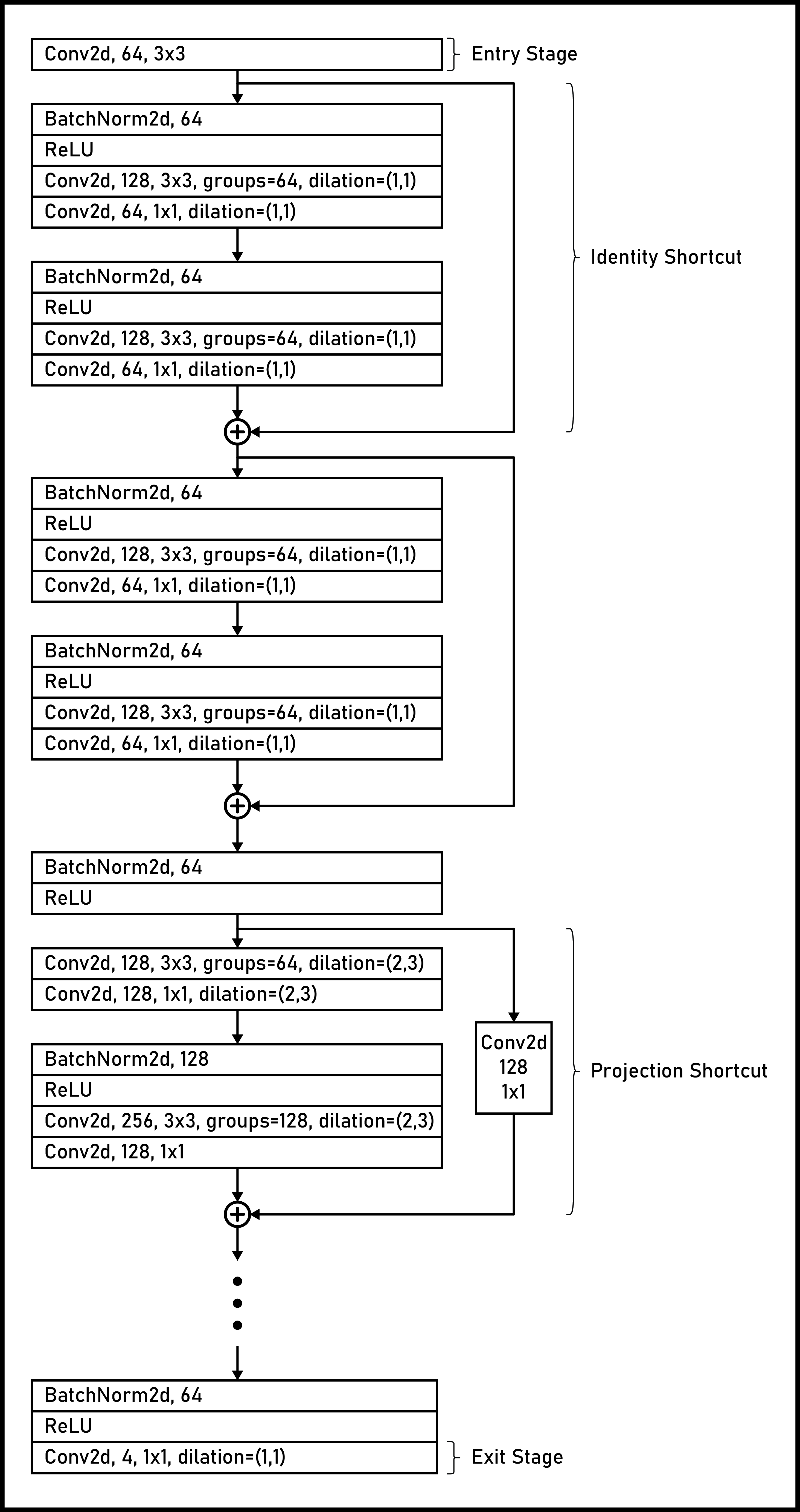
The AI-native fully convolutional receiver, DeepRx, uses a convolutional neural network (CNN) architecture that combines residual network (ResNet) blocks with full preactivation [2] and extreme inception (Xception) layers [3].
The network takes resource grids as input for an uplink (UL) single-input multiple-output (SIMO) system, where the grids have dimensions . The access node routes the grids through three main stages:
Entry stage — Receives the input grids.
Middle stage — Uses 11 residual network (ResNet) blocks with various dilation factors. Each block applies:
Identity shortcuts when input and output sizes match.
Projection shortcuts when sizes differ, enabling addition across blocks.
Depthwise separable convolutions to reduce computational complexity.
Exit stage — Applies batch normalization, ReLU, and a final convolution with an output size of .
This example uses a trained model (deeprx_30k.mat), which is included as a zipped supporting file in the example folder under the name torch_trained_network.zip.
For training details and solver settings, see the the AI-Native Fully Convolutional Receiver example. The following diagram shows the architectural flow of the AI-native fully convolutional receiver model.
Local Functions
function visualizePerformance(simParameters,resultsRX,resultsAIML)
    % Visualize the performance of the system by plotting coded BER and
    % throughput results against SNR for both MMSE based conventional 5G
    % and PyTorch AI-Native receiver

    % Create a figure object for the plots
    co = colororder;
    f = figure;
    f.Position(3:4) = [900 400];
    t = tiledlayout(1,2,TileSpacing="compact");

    % Plot coded BER against SNR
    nexttile;
    semilogy(simParameters.SNRInVec,[resultsAIML.CodedBER],"-*",Color=co(5,:),LineWidth=1.5,MarkerSize=7);
    hold on
    semilogy(simParameters.SNRInVec,[resultsRX.CodedBER],"-s",LineWidth=1.5,MarkerSize=7);
    hold off
    legend("DeepRx (PyTorch)","Conventional 5G Rx",Location="southwest");
    grid on;
    xlabel("SNR (dB)");
    ylabel("Coded BER");

    % Plot throughput against SNR
    nexttile;
    plot(simParameters.SNRInVec,[resultsAIML.PercThroughput],"-*",Color=co(5,:),LineWidth=1.5,MarkerSize=7);
    hold on
    plot(simParameters.SNRInVec,[resultsRX.PercThroughput],"-s",LineWidth=1.5,MarkerSize=7);
    hold off
    legend("DeepRx (PyTorch)","Conventional 5G Rx",Location="southeast");
    grid on;
    xlabel("SNR (dB)");
    ylabel("Throughput (%)");

    % Add title to tiled layout summarizing system configuration
    titleText = [displayParameters(simParameters), ' | Modulation: ', char(simParameters.ModulationType)];
    titleText = split(titleText,'DMRS ');
    titleText{2} = ['DMRS ', titleText{2}];
    title(t,titleText);
end

function [resultsRX,resultsTORCH] = compareReceiverPerformance(simParameters)
% Evaluate PUSCH link over SNR sweep
    simParameters.TrainNow    = false;
    simParameters.DisplayInfo = true;

    % Check if the Python execution mode is 'InProcess' with parallelism enabled
    if strcmp(simParameters.PythonExecutionMode,"InProcess") && simParameters.UseParallel
        error("Python execution mode must be OutOfProcess when UseParallel is true.")
    end

    % Preallocate the results
    resultsTORCH(1:length(simParameters.SNRInVec)) = ...
        struct( ...
        'SNRIn',           -1, ...
        'BLER',            -1, ...
        'UncodedBER',      -1, ...
        'CodedBER',        -1, ...
        'SimThroughput',   -1, ...
        'MaxThroughput',   -1, ...
        'PercThroughput',  -1 ...
        );

    resultsRX(1:length(simParameters.SNRInVec)) = ...
        struct( ...
        'SNRIn',           -1, ...
        'BLER',            -1, ...
        'UncodedBER',      -1, ...
        'CodedBER',        -1, ...
        'SimThroughput',   -1, ...
        'MaxThroughput',   -1, ...
        'PercThroughput',  -1 ...
        );

    % Simulation status
    border = repmat('_',1,40);
    fprintf('\n%s\n',border);
    fprintf('\nSimulating DeepRx and 5G receivers\n');
    fprintf('%s\n',border);

    % -----------------------------------------------------------------
    % Evaluate AI/DeepRx and conventional receivers over all SNR points
    % -----------------------------------------------------------------
    if simParameters.UseParallel && canUseParallelPool
        pool = gcp;
        maxWorkers = numel(simParameters.SNRInVec); % utilize each SNR point to a worker
        fprintf('\n- Test data generation: CPU acceleration on (%d) workers\n',pool.NumWorkers);
    else
        maxWorkers = 0; % serial execution
        fprintf('\n- Test data generation: Serial execution\n');
    end
    % Inference/prediction environment
    device = pyrun(["import torch", "device = torch.device('cuda:0' if torch.cuda.is_available() else 'cpu')"],"device");
    fprintf('- Inference environment: %s\n',upper(string(device.type)));
    fprintf('\nSimulating DeepRx and conventional receivers for %d SNR points...\n\n',numel(simParameters.SNRInVec));

    % -----------------------------------------------------------------
    % Each worker evaluates one SNR point (if enabled), otherwise
    % serial execution
    % -----------------------------------------------------------------
    parfor (i = 1:numel(simParameters.SNRInVec),maxWorkers)
        % Temporary parameter definitions for parfor
        simLocal = simParameters;
        simLocal.SNRIn = simParameters.SNRInVec(i);

        % End-to-end PUSCH simulation for each SNR point
        resultsRX(i) = hEvaluatePUSCHAtSNR(simLocal,Iteration=30e3+i+1);
        resultsTORCH(i) = hEvaluatePUSCHAtSNR(simLocal,Net="py.deeprx_model.DeepRx",Iteration=30e3+i+1);

        % Update progress status
        if simParameters.DisplayInfo
            fprintf(['SNRIn: %+6.2f dB | ',displayParameters(simParameters),'\n'],simLocal.SNRIn);
        end
    end
end

function dispText = displayParameters(simParameters)
% Display random/selected simulation parameters
    dispText = sprintf( ...
        ['Channel: %s | Delay spread: %-7.2e | Max Doppler shift: %-6.2f | ' ...
        'DMRS Add. Pos. / Config. Type: %d / %d'], ...
        simParameters.ChannelModel, ...
        simParameters.DelaySpread,simParameters.MaximumDopplerShift, ...
        simParameters.DMRSAdditionalPosition,simParameters.DMRSConfigurationType ...
        );
end

function displayNetworkSummary(modelParameters)
% Display network summary including layers and learnable parameters
    % Count layers using the LeNet-5 convention:
    % Convolution, pooling, and fully connected layers are counted.
    % Activation layers are not counted.

    % Convert model parameters to a cell array
    params = cell(modelParameters);

    % Extract and filter unique layer names
    layerNames = unique(string(params{2}),"stable");
    layerNames = layerNames(~ismember(layerNames, ["","bn","relu"]));

    % Print the network summary
    border = repmat('_',1,40);
    fprintf('\n%s\n',border);
    fprintf('\nNeural Network Summary\n');
    fprintf('%s\n\n',border);
    fprintf('%-28s: %.4f million\n', '- Total number of learnables',double(params{1})/1e6);
    fprintf('%-28s: %d\n', '- Number of layers',length(layerNames));
    fprintf('\n%-28s:\n', '- Model building blocks');

    % Display unique layerNames with aligned indices
    indexWidth = length(num2str(length(layerNames)));
    arrayfun(@(i) fprintf(['\t\t\t     %' num2str(indexWidth) 'd) %s\n'],i,layerNames{i}),1:length(layerNames));
end

function displayParameterSummary(simParameters)
    % Display the set of simulation parameters
    border = repmat('_',1,40);
    fprintf('\n%s\n', border);
    fprintf('\nSimulation Summary\n');
    fprintf('%s\n\n', border);
    fprintf('- %-33s [ %s ]\n', 'Input (X) size:',num2str(simParameters.InputSize));
    fprintf('- %-33s [ %s ]\n\n', 'Output (L) size:',num2str(simParameters.OutputSize));
    fprintf('- %-33s %-5d\n', 'Number of subcarriers (F):',simParameters.Carrier.NSizeGrid*12);
    fprintf('- %-33s %-5d\n', 'Number of symbols (S):',simParameters.Carrier.SymbolsPerSlot);
    fprintf('- %-33s %-5d\n', 'Number of receive antennas (Nrx):',simParameters.NRxAnts);
end

function simParameters = configureAIMLParameters(simParameters)
[~, info, ~] = nrPUSCHIndices(simParameters.Carrier,simParameters.PUSCH);
simParameters.NBits = info.G/info.Gd; % Number of bits

simParameters.InputSize  = [
    simParameters.Carrier.NSizeGrid*12, ...
    simParameters.Carrier.SymbolsPerSlot, ...
    4*simParameters.NRxAnts+2 ...
    ]; % DeepRx network input size [F S 4*Nr+2]

simParameters.OutputSize = [
    simParameters.Carrier.NSizeGrid*12, ...
    simParameters.Carrier.SymbolsPerSlot, ...
    simParameters.NBits ...
    ]; % DeepRx network output size
end
References
[1] M. Honkala, D. Korpi, and J. M. J. Huttunen, "DeepRx: Fully Convolutional Deep Learning Receiver," in IEEE Transactions on Wireless Communications, vol. 20, no. 6, pp. 3925—3940, June 2021.
[2] He, K., Zhang, X., Ren, S., and Sun, J., "Identity mappings in deep residual networks", in European Conference on Computer Vision, pp. 630—645, Springer, 2016.
[3] F. Chollet, "Xception: Deep Learning with Depthwise Separable Convolutions," in 2017 IEEE Conference on Computer Vision and Pattern Recognition (CVPR), Honolulu, HI, USA, 2017 pp. 1800—1807.