Design Log-Periodic Sawtooth Planar Antenna for UHF Ultra-Wideband Applications
This example shows how to create, model, and analyze two-arm log-periodic sawtooth planar microstrip antenna [1]. It is a bowtie-like antenna that consists of two arms located on the square-shaped FR4 dielectric substrate. This example designs a log-periodic sawtooth planar antenna with stable impedance over a wide bandwidth from 300 MHz to 1200 GHz. This antenna is widely used in the ultra high frequency (UHF) range and for ultra-wideband (UWB) systems such as ground penetrating radar systems (GPRs). The non-evasive and nondestructive technique in GPRs uses electromagnetic radiation in the microwave band. GPRs use high-frequency radio waves, usually in the 10 MHz to 2.6 GHz range.
Define Parameters
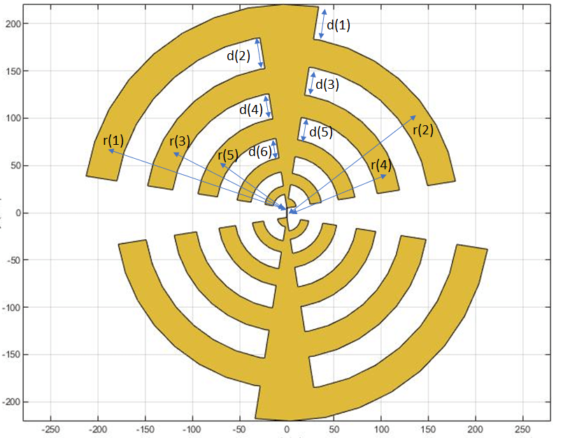
The dimensions and the variables used in this example are taken from the paper [1]. The variables r and d specify the radius and width of the arms of the log-periodic antenna. The Angle variable is used as an ArcAngle for creating the arms of the antenna. The r, d, and Angle variables are used to design the arms on either side of the center arc. The NumPoints variable is used to specify the number of discretization points.
Angle = 18;
r = [199 166 136 109 85 64 46 31 19 5]*1e-3;
d = [33  30  27  24  21 18 15 12 9 10]*1e-3;
NumPoints = 8;
Create Log-Periodic Shape
Use the generatePointsforCurve function to create the vertices for the arms of the antenna. This function takes the angle, radius, width, and number of discretization points as the inputs and generates the boundary vertices for the curves. These vertices are used to form an arm using the antenna.polygon function. All the arms on either side of the center arc can be generated by using r and d variables. All the polygons formed are combined to form the upper half of the log-periodic antenna.
NumShapes = numel(1,r);
p1 = generatePointsforCurve([90-Angle/2,90+Angle/2],(205e-3)/2,205e-3,NumPoints/2);
shp = antenna.Polygon(Vertices=p1');
for i=1:NumShapes
    if rem(i,2)==1
        tempPoints = generatePointsforCurve([90-Angle/2,180-Angle/2],r(i),d(i),NumPoints);
        tempShape = antenna.Polygon(Vertices=tempPoints');
        shp = shp + tempShape;
    else
        tempPoints = generatePointsforCurve([Angle/2,90+Angle/2],r(i),d(i),NumPoints);
        tempShape = antenna.Polygon(Vertices=tempPoints');
        shp = shp + tempShape;
    end
end
Shift the shape along the y-axis to create a gap for the feed using the translate function. The total gap given in [1] is 10 mm, so shift the upper half of the shape by 5 mm.
shp = translate(shp,[0 5e-3 0]);
Copy the shape into a variable shp1 and use it to create a symmetrical shape. Use the rotateZ function to rotate the shape replica by 180 degrees.
shp1 = copy(shp);
shp1 = rotateZ(shp1,180);
Create a rectangle for the feed 0.5 mm in length and 15 mm in width using the antenna.Rectangle shape object.
feed = antenna.Rectangle(Length=0.5e-3,Width=15e-3);
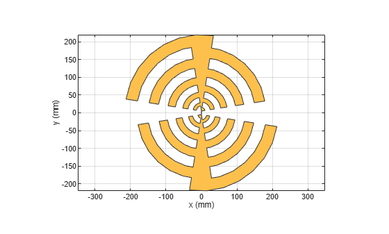
Unify shapes shp and shp1 with the feed to form sawtooth-shaped antenna structure.
shape = shp + shp1 + feed;
figure
show(shape)
Create Log-Periodic Antenna Using PCB Stack
Create a pcbStack object with two layers. The top metal layer is the log-periodic shape antenna and the bottom layer is the square-shaped dielectric substrate FR4 of length 470 mm. The substrate has a dielectric constant of 4.6, an attenuation coefficient of 0.02, and the substrate thickness of 1.6 mm. The top conductor is set to copper with a thickness of 35 um.
ant = pcbStack;
d = dielectric("FR4");
d.Thickness = 1.6e-3;
d.FrequencyModel = "DjordjevicSarkar";
ant.BoardThickness = 1.6e-3;
BoardDim = antenna.Rectangle(Length=470e-3,Width=470e-3);
ant.Name = "LogPeriodic";
ant.Layers = {shape,d};
ant.BoardShape = BoardDim;
ant.FeedLocations = [0 0 1];
ant.FeedDiameter = 0.25e-3;
ant.FeedViaModel = "strip";
ant.Conductor = metal("copper");
ant.Conductor.Thickness = 35e-6;
Use the show function to visualize the antenna.
figure
show(ant)
title("Log-Periodic Sawtooth Planar Antenna")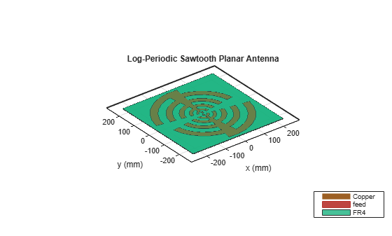
Mesh Antenna Structure
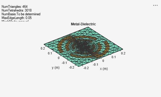
Mesh the structure by specifying the maximum edge length. Below is the mesh used to model the antenna. The triangles are used to discretize the metal regions of the patch, and tetrahedra are used to discretize the volume of the dielectric substrate in the antenna. The triangles and tetrahedra are indicated by the colors yellow and green, respectively. The total number of unknowns is the sum of the unknowns for the metal plus the unknowns used for the dielectric. As a result, the time to calculate the solution increases significantly as compared to pure metal antennas. Set the maximum edge length to 0.05. This value can be decreased to generate a denser mesh.
figure
mesh(ant,MaxEdgeLength=0.05)
Analyze Antenna
Plot the impedance of the antenna using the impedance function over a frequency range of 100-1250 MHz.
figure
impedance(ant,100e6:10e6:1250e6);
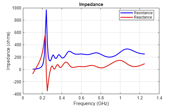
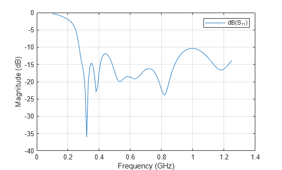
The impedance plot shows that real part of the impedance is approximately 220 ohms over the specified range. And the imaginary part of the impedance is almost 0. The results in [1] are obtained by using a balun to transform the impedance to 50 ohms. Set the reference impedance as 220 ohms to obtain results similar to [1]. Plot S-parameters over a frequency 300-1250MHz with the reference impedance of 220 ohms using the sparameters function. The antenna has an S11 of value less than -10 dB over a frequency range of 300-1200 MHz.
spar = sparameters(ant,100e6:10e6:1250e6,220);
figure
rfplot(spar)
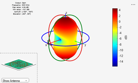
Use the pattern function to plot the radiation pattern of the antenna at a frequency of 600 MHz.
figure
pattern(ant,600e6)
Plot the radiation pattern of the antenna in the rectangular cartesian coordinate system over a frequency range of 300-1200 MHz
figure
pattern(ant,300e6:100e6:1200e6,0,90,CoordinateSystem="rectangular")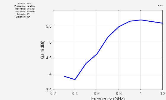
Conclusion
Modeling and analysis of a log-periodic antenna using the Antenna Toolbox is completed and its performance matches the results given in [1]. The return loss (S11) of the antenna indicates a wideband performance over a frequency range of 300-1200 MHz. The antenna has an approximate gain of 4.65 dBi at 600 MHz and the gain increases with the increase in frequency.
Reference
[1]. Phu B. H., Quang P. M., Phuoc D. T. and Duy L. N., "A log-periodic saw-toothed planar antenna for UHF ultra-wideband applications," 2013 International Conference on Advanced Technologies for Communications, 2013, pp. 689-692.