Anomaly Detection in Signal Labeler Using Time-Series Foundation Model
This example shows how to integrate a Chronos model [1] into a MATLAB® workflow to detect anomalies in signals. The example also shows how to use the Chronos model as a custom labeling function in Signal Labeler and then use Signal Labeler to label the anomalous regions.
Introduction
Chronos is a pretrained foundation model that you can use for probabilistic time-series forecasting. Foundation models like Chronos can handle a wide range of time-series forecasting tasks with minimal customization. You can apply the model to a data set without training it on that data set and adapt it for tasks such as anomaly detection and imputation.
In this example, you implement the model in PyTorch®. The chronos_forecast.py file defines the interface functions to load Chronos models and perform forecasting. The helperReconstructSignalWithChronos function handles data exchange between MATLAB and Python®, using the Chronos forecasting model to reconstruct the full signal from overlapping segments. By comparing the reconstructed signal with the observed data and thresholding the reconstruction error, this anomaly detection approach identifies regions that deviate significantly from model expectations as anomalies. The helperCustomDetectAnomalies helper function integrates Chronos as a custom auto labeling function in Signal Labeler, allowing automatic preliminary labeling of suspicious regions for manual review.
Set Up Python Environment
Chronos is implemented in PyTorch, so you must configure a Python environment for MATLAB to call. To install a supported Python implementation, see Configure Your System to Use Python. To avoid library conflicts, use the External Languages side panel in MATLAB to create a Python virtual environment using the requirements_chronos.txt file. For details on the External Languages side panel, see Manage Python Environments Using External Languages Panel. For details on Python environment execution modes and debugging Python from MATLAB, see Python Coexecution.
Use the helperCheckPyenv function to verify that the current PythonEnvironment contains the libraries listed in the requirements_chronos.txt file. This example was tested using Python 3.11.2.
requirementsFile = "requirements_chronos.txt";
currentPyenv = helperCheckPyenv(requirementsFile,Verbose=true);
Checking Python environment Parsing requirements_chronos.txt Checking required package 'chronos-forecasting' Checking required package 'torch' Required Python libraries are installed.
You can use the following process ID and name to attach a debugger to the Python interface and debug the example code.
fprintf("Process ID for '%s' is %s.\n", ...
  currentPyenv.ProcessName,currentPyenv.ProcessID)
Process ID for 'MATLABPyHost' is 2955697.
Chronos is available in multiple pretrained variants, such as chronos-t5-tiny, chronos-t5-small, and larger models. You can choose a variant depending on the complexity of your task and available resources. The actual pretrained model is not loaded into memory until you make the first prediction using that model name.
Detect Anomalies Using Chronos from MATLAB
Prepare Signal with Injected Anomaly
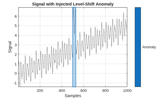
Create a synthetic time series with smooth oscillations and add a level-shift anomaly over a short interval.
rng("default");

T = 1000;
t = (0:T-1)';

base = sin(2*pi*t/20).*(1 + 0.5*sin(2*pi*t/50));
signal = base + 0.1*randn(T,1)+t/200;
st = 500;
dur = 30;
anomalyMask = false(T,1);
signal(st:st+dur-1) = signal(st:st+dur-1) + 3;
anomalyMask(st:st+dur-1) = true;
At this point, signal contains a localized anomaly, and anomalyMask records the ground truth for that anomaly region.
Convert the logical anomaly mask to a signalMask object and plot it over the signal. The shaded region highlights samples marked as anomalous.
msk = signalMask(anomalyMask,Categories="Anomaly");
figure
plotsigroi(msk,signal,true);
title("Signal with Injected Level-Shift Anomaly")
xlabel("Samples")
ylabel("Signal")
grid on
Reconstruct Signal Using Chronos
Use the helperReconstructSignalWithChronos helper function to call the Chronos model from MATLAB. For this case, use the lightweight chronos-t5-tiny variant.
Chronos is a probabilistic forecaster that not only provides a single reconstructed signal but also produces uncertainty bounds. The helperReconstructSignalWithChronos helper function returns a median prediction (recon) and lower and upper bounds (reconlow and reconhigh) that define a central 80% confidence band, giving a sense of confidence around the predicted signal.
Modify the function parameters to control how the function reconstructs the signal.
ContextLength— Control the number of previous time steps to use.MaxHorizon— Determine how far ahead to predict at each window.Stride— Set the step size between forecast windows.ModelName— Select the Chronos model to use. The lightweight"amazon/chronos-t5-tiny"runs quickly, while"amazon/chronos-t5-small"or"amazon/chronos-t5-base"can improve accuracy on more complex data.ExecutionEnvironment— Specify the hardware resource for running the model. Defaults to "auto", but can be set to "cpu" or "gpu" for explicit control.Verbose— Control whether to display detailed progress information.
The helper function internally slides a context window along the signal, forecasts MaxHorizon samples at each step using Chronos, and assembles the forecasts into full-length outputs.
[recon, reconlow, reconhigh] = helperReconstructSignalWithChronos( ...
    signal, ...
    ContextLength=256, ...
    MaxHorizon=32, ...
    Stride=8, ...
    ModelName="amazon/chronos-t5-tiny", ...
    ExecutionEnvironment="auto", ...
    Verbose=true);
[MATLAB] Clearing pipeline cache...
[chronos] pipeline cache cleared
[MATLAB] Starting forward reconstruction: 90 windows (aggregation: mean)
[chronos] initializing pipeline with ('amazon/chronos-t5-tiny', 'auto', torch.float32)
[MATLAB] 1/90 forward window | elapsed=0.7s ETA=59.8s
[MATLAB] 10/90 forward window | elapsed=3.0s ETA=24.0s
[MATLAB] 20/90 forward window | elapsed=5.6s ETA=19.6s
[MATLAB] 30/90 forward window | elapsed=8.2s ETA=16.4s
[MATLAB] 40/90 forward window | elapsed=10.7s ETA=13.4s
[MATLAB] 50/90 forward window | elapsed=13.3s ETA=10.6s
[MATLAB] 60/90 forward window | elapsed=15.8s ETA=7.9s
[MATLAB] 70/90 forward window | elapsed=18.4s ETA=5.3s
[MATLAB] 80/90 forward window | elapsed=21.0s ETA=2.6s
[MATLAB] 90/90 forward window | elapsed=23.6s ETA=0.0s
Compute Anomaly Scores and Detect Anomalies
Compute an uncertainty-aware score by dividing the absolute reconstruction error by the predictive band half-width. A narrow band implies high confidence, so small errors count more, and a wide band reduces their influence. Set the threshold to a high quantile of the valid scores and flag samples above it as anomalies.
bandhalf = max(0.5*(reconhigh - reconlow),1e-6);
score = abs(signal - recon)./bandhalf;
valid = isfinite(score);
globalthresh = quantile(score(valid),0.95);
detected = false(size(score));
detected(valid) = score(valid) > globalthresh;
fprintf("Score stats (valid), min=%.3f, median=%.3f, max=%.3f, thresh=%.3f\n", ...
    min(score(valid)), median(score(valid)), max(score(valid)), globalthresh);
Score stats (valid), min=0.001, median=0.550, max=6.351, thresh=2.089
Visualize Results
Show the signal with ground truth and detected regions. Plot the score with the threshold.
mskTruth = signalMask(anomalyMask,Categories="truth");
mskDet = signalMask(detected,Categories="detected",MinLength=10,MergeDistance=10);

fig = helperPlotAnomalyResults(t, signal, recon, score, mskTruth, mskDet, ...
    Threshold=globalthresh, ...
    ReconLow=reconlow, ...
    ReconHigh=reconhigh, ...
    ValidIdx=valid);
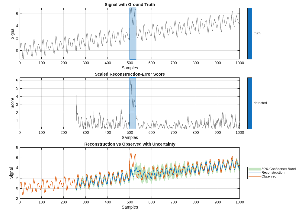
From the plots, you can see that reconstruction tracks the normal pattern when the signal is healthy. The confidence band becomes wider near the anomaly, which means the model is less sure about what comes next.
The detected region starts with the true anomaly, and the score rises quickly after the change and stays low elsewhere. After the anomaly, the higher uncertainty makes it hard for the model to tell exactly when the signal is back to normal. In practice, you can refine the exact start and end and the type by hand. But, on large data sets the automatic detector can flag likely anomalous intervals and save a lot of manual work.
Use Chronos as Custom Labeling Function in Signal Labeler
You can use the same reconstruction-based anomaly score to assign preliminary labels to anomalous regions in the Signal Labeler app. The custom labeling function helps you quickly mark suspected anomalies and then adjust them manually, which reduces labeling effort and supports assisted labeling.
Generate example data with five signals, where the first three include injected anomalies:
helperCreateSignals
Signal 1/5: type=dropout, length=1000
Signal 2/5: type=level_shift, length=800
Signal 3/5: type=noise_burst, length=1200
Signal 4/5: type=normal, length=950
Signal 5/5: type=normal, length=1100
Open Signal Labeler.
signalLabeler
Complete the following steps in Signal Labeler:
In the File section of the Labeler tab, click Import and select From Workspace to import
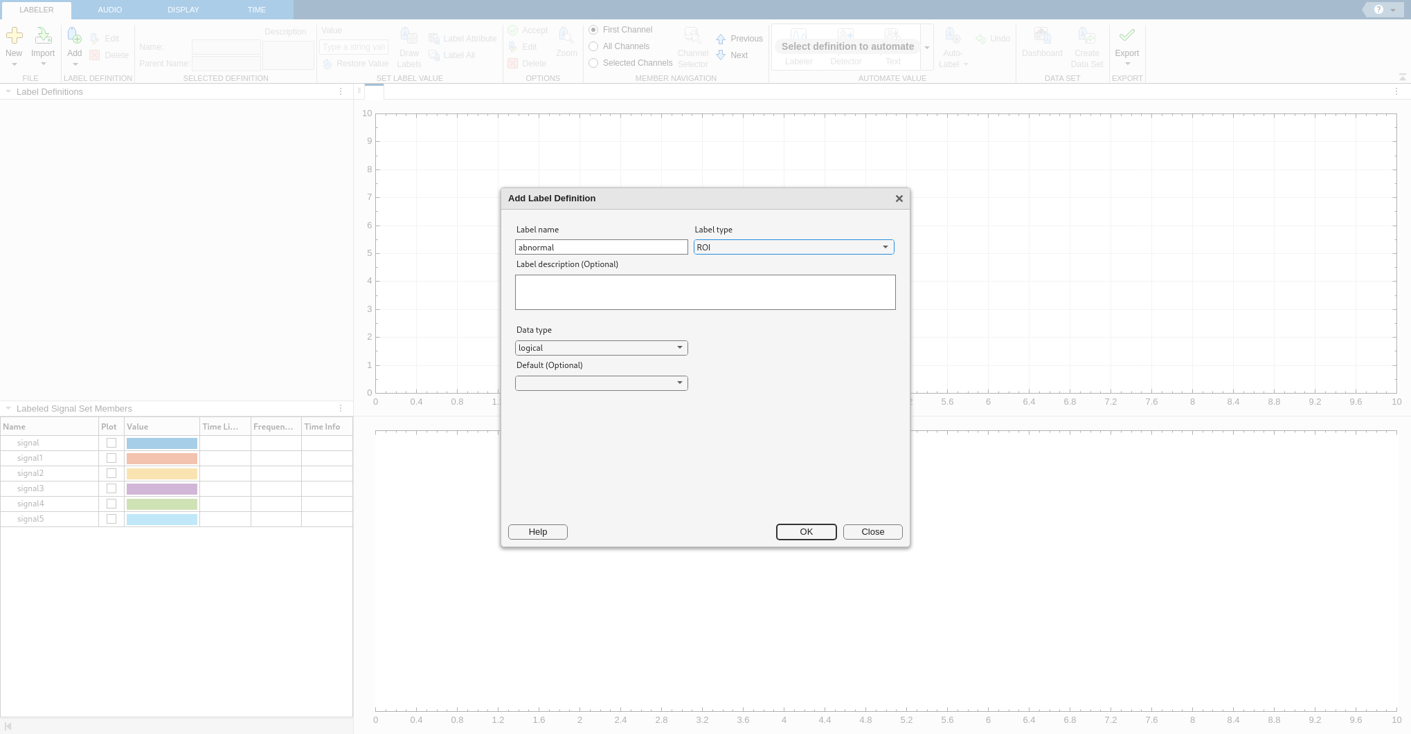
signal1–signal5into Signal Labeler.In the Label Definition section of the Labeler tab, click Add and select Add Label Definition. In the dialog box that appears, set label name to
abnormaland label type toROI.
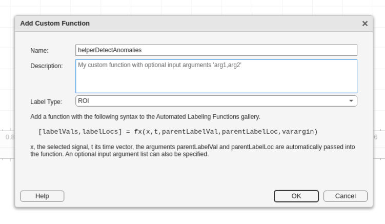
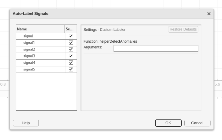
Create a custom labeling function using the Chronos-based detector helperCustomDetectAnomalies helper function.
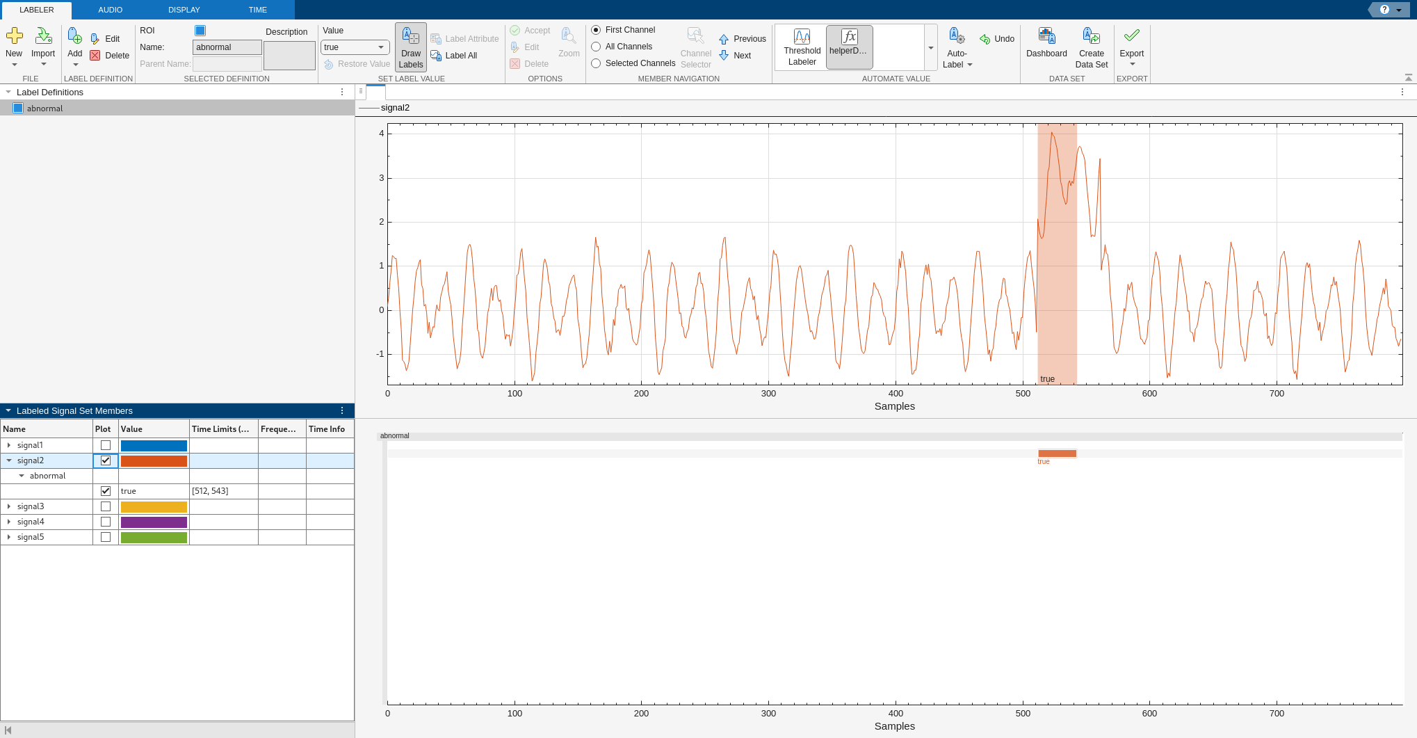
In the Automate Value section of the Labeler tab, click Auto-Label and choose Auto-Label All Signals. In the dialog box that appears, select the signals.
For instance, the autolabeled ROI in signal2 aligns with the true anomalous region and is ready for manual adjustment.
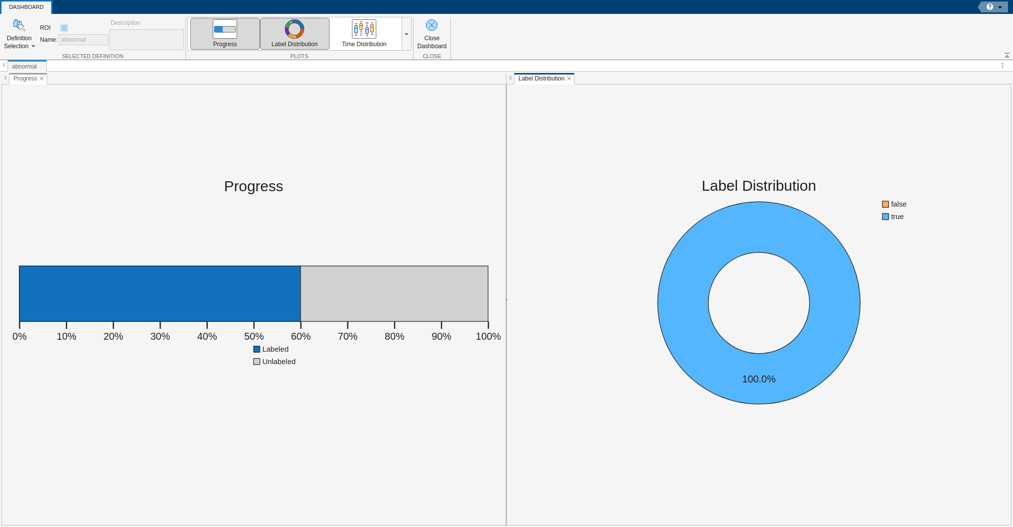
From the dashboard you can see that three of five signals are labeled true, meaning they contain anomalies. The result in the dashboard matches how the data was generated with three anomalous signals. The custom function applies preliminary labels so you can focus your review on only those three signals instead of the full data set and open each signal to adjust the ROI start and end times or further set the anomaly type.
Conclusion
This example shows how to integrate a time-series foundation model implemented in Python into MATLAB workflows and Signal Labeler, enabling reconstruction-based anomaly detection and assisted labeling directly within MATLAB. By bringing Chronos and other Python capabilities into MATLAB, you can expand detection and labeling options while continuing to leverage MATLAB interactive apps, visualization, and analysis tools in a seamless environment.
Reference
[1] Ansari, Abdul Fatir, Lorenzo Stella, Caner Turkmen, Zhang Xiyuan, Pedro Mercado, Huibin Shen, Oleksandr Shchur, et al. "Chronos: Learning the Language of Time Series." Transactions on Machine Learning Research, 2024. https://openreview.net/forum?id=gerNCVqqtR
Appendix — Helper Functions
helperPlotAnomalyResults This function plots anomaly detection results with reconstruction and uncertainty.
function fig = helperPlotAnomalyResults(t, signal, recon, score, mskTruth, mskDet, options)
% This function is only intended to support this example. It may be changed
% or removed in a future release.

    arguments
        t (:,1) {mustBeNumeric}
        signal (:,1) {mustBeNumeric}
        recon (:,1) {mustBeNumeric}
        score (:,1) {mustBeNumeric}
        mskTruth
        mskDet
        options.ReconLow (:,1) {mustBeNumeric} = []
        options.ReconHigh (:,1) {mustBeNumeric} = []
        options.ValidIdx (:,1) logical = true(size(t))
        options.Threshold (1,1) {mustBeNumeric} = []
    end

    fig = figure(Position=[100 100 1000 700]);
    tiledlayout(3, 1, TileSpacing="compact", Padding="compact")

    % Plot 1: Signal with Ground Truth
    nexttile
    plotsigroi(mskTruth, signal, true)
    title("Signal with Ground Truth")
    xlabel("Samples")
    ylabel("Signal")
    grid on
    box on

    % Plot 2: Scaled Reconstruction-Error Score
    nexttile
    plotsigroi(mskDet, score, true)
    hold on
    yline(options.Threshold, "--")

    title("Scaled Reconstruction-Error Score")
    xlabel("Samples")
    ylabel("Score")
    grid on
    box on
    hold off

    % Plot 3: Reconstruction vs Observed with Uncertainty
    nexttile
    hold on
    if ~isempty(options.ReconLow) && ~isempty(options.ReconHigh)
        x = t(options.ValidIdx);
        ylow = options.ReconLow(options.ValidIdx);
        yhigh = options.ReconHigh(options.ValidIdx);
        co = get(gca, "ColorOrder");
        c = co(5, :);
        fill([x; flipud(x)], [ylow; flipud(yhigh)], c, ...
            EdgeColor="none", FaceAlpha=0.3, ...
            DisplayName="80% Confidence Band")
    end
    plot(t, recon, LineWidth=1.2, DisplayName="Reconstruction")
    plot(t, signal, LineWidth=0.8, DisplayName="Observed")
    title("Reconstruction vs Observed with Uncertainty")
    xlabel("Samples")
    ylabel("Signal")
    legend(Location="eastoutside")
    grid on
    box on
    hold off

    linkaxes(findall(fig, Type="axes"), "x")

end