Comfort Distance and Distraction Distance (ISO 3382-3)

Since R2026a

This example demonstrates how to compute the single-number quantities comfort distance ( $r_{C}$ ) and distraction distance ( $r_{D}$ ) for an open-plan office following the ISO 3382-3:2022 standard [1]. The workflow mirrors the standard:

Build a simple geometric office model with furniture to emulate scattering/occlusions.
Place an omnidirectional sound source (OSS) and receivers along a linear measurement path, at heights and spacings consistent with the standard.
Simulate the required measurements: distances from OSS to receivers, octave-band SPLs at receivers with and without OSS, and room impulse responses (RIRs) at receivers for speech transmission index (STI) computation.
Derive the spatial decay rate of A-weighted speech per distance doubling ( $D_{2, S}$ ), the A-weighted speech level at 4 m ( $L_{p, A, S, 4 m}$ ), and comfort distance $r_{C}$ using ISO 3382-3 formulas.
Define STI as a function of distance and derive the distraction distance $r_{D}$ by linear regression to the point STI = 0.50.

Model Room

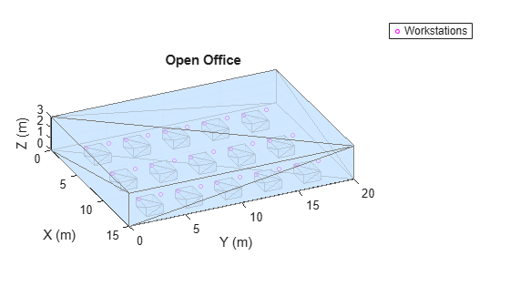
Model the room as a 15 meter (width) by 20 meter (length) by 3 meter (height) space. Use the supporting function iCreateRoom to create a triangulation object using the room dimensions and fill it with tables representing workstations. Use the supporting function iPlotRoom to visualize the room.

roomdims = [15,20,3];

[room,workstationLocations] = iCreateRoom(roomdims);
iPlotRoom(room,workstationLocations)

Figure contains an axes object. The axes object with title Open Office, xlabel X (m), ylabel Y (m) contains 2 objects of type patch, line. One or more of the lines displays its values using only markers This object represents Workstations.

Simulate Measurements

Simulate standard-compliant measurement locations. The OSS is placed at the prescribed 1.2 m height at a workstation at one end of the measurement path. Receivers are placed on a straight line away from the OSS, also at 1.2 m height, at each workstation. The standard states that there should be at least four successive measurement positions on the path and that the preferred number of positions is six to ten. Measurements of receivers greater than 16 m from the source are not necessary.

A room should be divided in distinct acoustic zones, if they exist, and resulting metrics should be calculated and reported independently. Within a single acoustic zone, at least two separate measurement paths should be taken and the results averaged. If only one path exists in an acoustic zone, both directions of the path should be taken and averaged. This example walks through the computations for a single measurement path. In section Measure Multiple Paths, another path is simulated and measured and the results averaged for reporting. See [1] for further details on compliant procedures.

Define the OSS position and receiver positions in the room and visualize.

tx = [8,1.75,1.2];
rx = [8,3.75,1.2;
    8,5.25,1.2;
    8,7.25,1.2;
    8,8.75,1.2;
    8,10.75,1.2;
    8,12.25,1.2;
    8,14.25,1.2;
    8,15.75,1.2;
    8,17.75,1.2];

iPlotRoom(room,workstationLocations,tx,rx)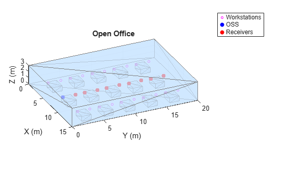

Figure contains an axes object. The axes object with title Open Office, xlabel X (m), ylabel Y (m) contains 4 objects of type patch, line. One or more of the lines displays its values using only markers These objects represent Workstations, OSS, Receivers.

Calculation of comfort distance and distraction distance require the following measurements at each receiver location:

Distance to the OSS disregarding the obstacles, r
Unweighted equivalent SPL of wide-band noise produced by the OSS, $L_{p, tot}$
Unweighted equivalent SPL of background noise, $L_{p, B}$
Room impulse response for the calculation of the speech transmission index (STI)

Calculate the straight-line distance in meters.

r_n = vecnorm(rx - tx,2,2);

Simulate the SPL measurement of the OSS at 1 m distance. Use a plausible level (80 dB per band) with a small random variation.

rng default
L_poss1mff_base = 80*ones(1,7);
L_poss1mff_jitter = 4;
L_poss1mff = L_poss1mff_base + (L_poss1mff_jitter*(rand(1,7) - 0.5));

Simulate the SPL measurement at each receiver using a simple inverse distance decay formulation. Free-field decay is typically set to 6 dB per doubling. Add mild spatial variability to model furniture/screening and room effects.

d0 = 1; % reference distance in meters
decayPerDoubling = 5.8;
ossSpatialJitter = 6;
L_ptot = L_poss1mff - decayPerDoubling*log2(r_n./d0) + (ossSpatialJitter*(rand(numel(r_n),7) - 0.5)); % numReceiver x octave SPL

Simulate background noise measured at each position. A pink noise shape is typical. Add variability to the measurement.

L_pB_base = [44,41,38,35,32,29,26];
L_pB_jitter = 6;
L_pB = L_pB_base + (L_pB_jitter*(rand(numel(r_n),7) - 0.5)); % numReceiver x octave SPL

To simulate RIR at each measurement location, use acousticRoomResponse and specify the room triangulation object, the source location, and the receiver locations.

fs = 48e3;
rir = acousticRoomResponse(room,tx,rx,SampleRate=fs); % numReceiver x rir length

Add a noise floor to mimic real measurements.

noiseFloor = -60;
rir = iAddNoiseFloor(rir,fs,noiseFloor);

Spatial Decay Rate of Speech

In this section, you determine the attenuation of the broadband noise output from the omnidirectional sound source and apply that attenuation to an average speech spectrum to estimate the speech levels at each receiver.

Apply background noise correction to the SPL of the OSS according to formula 3 of [1]:

$L_{p, oss} = 10 {\cdot \log}_{10} (10^{\frac{L_{p, tot}}{10}} - 10^{\frac{L_{p, B}}{10}})$

where

$L_{p, oss}$ is the background noise-corrected SPL of OSS in dB.
$L_{p, B}$ is the SPL of background noise (OSS is off) in dB.
$L_{p, tot}$ is the measured SPL in dB, which includes both background noise and the wide-band noise produced by the OSS.

L_poss = pow2db(db2pow(L_ptot) - db2pow(L_pB));

Calculate the attenuation $D_{n, i}$ (dB) of wide-band noise at the measurement position $n$ at distance $r_{n}$ according to formula 2 of [1]:

$D_{n, i} = L_{p, oss, 1 m, ff, i} - L_{p, oss, n, i}$

where

$L_{p, oss, 1 m, ff, i}$ is the background-noise corrected SPL of the OSS at 1.0 m distance in free field.
$L_{p, oss, n, i}$ is the measured SPL produced by the OSS at position $n$ .

D_ni = L_poss1mff - L_poss;

The SPL of normal effort speech, $L_{p, S, n, i}$ , at measurement position $n$ is according to formula 4 of [1]:

$L_{p, S, n, i} = L_{p, S, 1 m, ff, i} - D_{n, i}$ ,

where $L_{p, S, 1 m, ff, i}$ is the SPL of normal speech in a free field at 1 m distance from the OSS.

L_pS1mffi = [49.9,54.3,58.0,52.0,44.8,38.8,33.5]; % Given from table 1
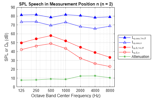
L_pSni = L_pS1mffi - D_ni;

Recreate figure 2 from ISO 3382-3. The calculated attenuation of the speech spectrum matches the measured OSS attenuation.

figure
n = 2;
cf = [125,250,500,1000,2000,4000,8000];
semilogx(cf,L_poss1mff,"-^b",MarkerFaceColor="b")
hold on
plot(cf,L_poss(n,:),"-^b")
plot(cf,L_pS1mffi,"-or",MarkerFaceColor="r")
plot(cf,L_pSni(n,:),"-or")
plot(cf,L_poss1mff - L_poss(n,:),"-*")
xlabel("Octave Band Center Frequency (Hz)")
ylabel("SPL or D_{n} (dB)")
grid on
ylim([0,90])
legend("L_{p,oss,1m,ff}","L_{p,oss,n}","L_{p,S,1m,ff}","L_{p,S,n}","Attenuation", Location="eastoutside")
title("SPL Speech in Measurement Position n (n = " + n + ")")
xticks([125,250,500,1000,2000,4000,8000])
hold off

$Figure contains an axes object. The axes object with title SPL Speech in Measurement Position n (n = 2), xlabel Octave Band Center Frequency (Hz), ylabel SPL or D indexOf n baseline (dB) contains 5 objects of type line. These objects represent L_{p,oss,1m,ff}, L_{p,oss,n}, L_{p,S,1m,ff}, L_{p,S,n}, Attenuation.$

Comfort Distance

Comfort distance describes the effect of spatial attenuation in an office without consideration of speech privacy, background noise level, or sound masking. A lower comfort distance indicates that the speech sound level decays more quickly with distance (greater attenuation), which generally results in more acoustic comfort for workstations surrounding the speaker.

Calculate the overall A-weighted SPL of speech in position $n$ , $L_{p, A, S, n}$ , according to formula 5 of [1]:

$L_{p, A, S, n} = 10 \cdot \log_{10} (\sum_{i = 1}^{7} 10^{\frac{L_{p, S, n, i} + A_{i}}{10}})$

where $A_{i}$ is the A-weighting vector given in Table 1 of [1].

Ai = [-16.1,-8.6,-3.2,0.0,1.2,1.0,-1.1];
L_pASn = pow2db(sum(db2pow(L_pSni + Ai),2));

Calculate the rate of spatial decay of A-weighted SPL of speech per doubling in decibels according to formula 6 of [1]:

$D_{2, S} = - \log_{10} (2) \cdot (\frac{N \sum_{n = 1}^{N} [L_{p, A, S, n} \cdot \log_{10} (\frac{r_{n}}{r_{0}})] - [\sum_{n = 1}^{N} L_{p, A, S, n}] \cdot [\sum_{n = 1}^{N} \log_{10} (\frac{r_{n}}{r_{0}})]}{N \sum_{n = 1}^{N} {[\log_{10} (\frac{r_{n}}{r_{0}})]}^{2} - {[\sum_{n = 1}^{N} \log_{10} (\frac{r_{n}}{r_{0}})]}^{2}})$

where

$L_{p, A, S, n}$ is the A-weighted SPL of speech in measurement position $n$ .
$N$ is the total number of measurement positions within distance range 2 m to 16 m.
$r_{n}$ is the distance from the middle point of the OSS to the measurement position $n$ .
$r_{0}$ is a constant reference distance, $r_{0} = 1.0 m$ .

fitmask = r_n >= 2 & r_n <= 16;
L_pASn_masked = L_pASn(fitmask);
r_n_masked = r_n(fitmask);

r0 = 1;
N = numel(r_n_masked);
num = N*sum(L_pASn_masked.*log10(r_n_masked/r0)) - sum(L_pASn_masked)*sum(log10(r_n_masked/r0));
denom = N*sum(log10(r_n_masked/r0).^2) - sum(log10(r_n_masked/r0)).^2;
D_2S = -log10(2)*(num/denom);

Calculate the speech level at 4 m distance. $L_{p, A, S, 4 m}$ according to formula 7 of [1]:

$L_{p, A, S, 4 m} = \frac{1}{N} \sum_{n = 1}^{N} L_{p, A, S, n} + D_{2, S} \cdot \frac{1}{N} \sum_{n = 1}^{N} \log_{2} (\frac{r_{n}}{4})$

L_pAS4m = mean(L_pASn_masked) + D_2S*mean(log2(r_n_masked/4));

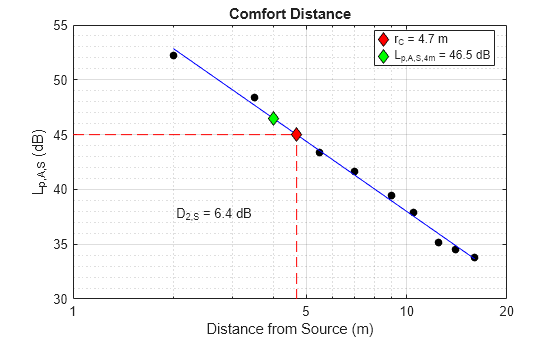
Calculate comfort distance according to formula 8 of [1]:

$r_{C} = 2^{\frac{(L_{p, A, S, 4 m} - 45 + 2 \cdot D_{2, S})}{D_{2, S}}}$

r_C = 2^((L_pAS4m - 45 + 2*D_2S)/D_2S)

r_C = 
4.6809

The ISO 3382-3 standard provides the following guidance for edge cases:

If $L_{p, A, S, n}$ is below 45 dB at the first measurement position, $r_{C}$ is determined by extrapolation and shall be stated as smaller than the distance to the first position.
If $L_{p, A, S, n}$ is above 45 dB at the remotest position, $r_{C}$ is determined by extrapolation and shall be stated as larger than the distance to the remotest position.

Verify neither of these edges cases apply.

useExtrapolation = (L_pASn_masked(1) < 45) || (L_pASn_masked(end) > 45)

useExtrapolation = logical
   0

Visualize the measurements, $L_{p, A, S, 4 m}$ , and comfort distance $r_{C}$ .

figure

semilogx(r_n,L_pASn,"ok",MarkerFaceColor="k",MarkerSize=5);
hold on
xlabel("Distance from Source (m)")
ylabel("L_{p,A,S} (dB)")

grid on
grid minor

xlim([1,20])
xticks([1,5,10,20])

% Plot fit line
x = log2(r_n_masked/r0);
a = mean(L_pASn_masked) + D_2S * mean(x);
yfit = a - D_2S*log2(r_n_masked/r0);
plot(r_n_masked,yfit,"b-",LineWidth=0.1)

% Plot comfort distance threshold (45 dB)
plot([1,r_C],[45 45],"--r",LineWidth=0.1)
plot([r_C,r_C],[30 45],"--r",LineWidth=0.1)

% Mark comfort distance
h1 = plot(r_C,45,"dk",MarkerFaceColor="r",MarkerSize=7);
h2 = plot(4,L_pAS4m,"dk",MarkerFaceColor="g",MarkerSize=7);

legend([h1,h2],sprintf('r_C = %0.1f m',r_C),sprintf('L_{p,A,S,4m} = %0.1f dB',L_pAS4m),Location="best")
title("Comfort Distance")

annotation("textbox",String=sprintf('D_{2,S} = %0.1f dB',D_2S),EdgeColor="none")
hold off

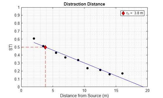
$Figure contains an axes object. The axes object with title Comfort Distance, xlabel Distance from Source (m), ylabel L indexOf p,A,S baseline (dB) contains 6 objects of type line. One or more of the lines displays its values using only markers These objects represent r_C = 4.7 m, L_{p,A,S,4m} = 46.5 dB.$

Distraction Distance

Distraction distance describes the combined effect of spatial attenuation and background noise level in an office, as it relates to speech privacy. A lower distraction distance indicates that the intelligibility of speech (as measured by STI) falls below the threshold for distraction more quickly with distance, which generally results in more speech privacy and less distraction for workstations surrounding the speaker.

To compute the speech transmission index (STI) at each location, use speechTransmissionIndex. Specify the measured RIR, sample rate of simulation, and operational signal and noise levels ( $L_{p, S, n, i}$ and $L_{p, B}$ ) at the receivers. Per the standard, specify the background noise level as the average over every measurement position along the measurement path. Spatial variation of the background noise level along the measurement path can increase direction dependent difference of $r_{D}$ and this situation is avoided by taking the average over the measurement positions. If more than one path is used, average across all paths. If only one path is used, average over the two opposite directions of that path for reporting. The standard also states that the speech transmission index for public address systems (STIPA) shall not be used to replace STI measurements. The default configuration of speechTransmissionIndex is compliant with IEC 60268-16:2020 and ISO 3382-3.

L_pB_avg = mean(L_pB,1);

sti = nan(numel(r_n),1);
for ii = 1:size(rir,1)
    sti(ii) = speechTransmissionIndex(rir(ii,:),fs, ...
        OperationalSignalLevel=L_pSni(ii,:), ...
        OperationalNoiseLevel=L_pB_avg);
end

Determine a linear fit and then derive the distraction distance (when the linear fit intersects with an STI of 0.5). All reference positions are used for the calculation except the reference position at 1 m distance.

sti_fit = polyfit(r_n, sti, 1);
yfit = polyval(sti_fit, [r_n;20]);
r_D = (0.50 - sti_fit(2)) / sti_fit(1);

Plot the distraction distance. This figure mimics figure 3 b from the 3382-3 standard.

figure
plot(r_n,sti,"ok",MarkerFaceColor="k",MarkerSize=5)

grid on
grid minor
xlabel("Distance from Source (m)")
ylabel("STI")
hold on
plot([r_n;20],yfit,"b-")
plot([0;r_D],[0.5,0.5],"--r",LineWidth=0.1)
plot([r_D;r_D],[0,0.5],"--r",LineWidth=0.1)
title("Distraction Distance")

h = plot(r_D,0.5,"dk",MarkerFaceColor="r",MarkerSize=7);

ylim([0,1])

legend(h,sprintf("r_D =  %0.1f m",r_D))
hold off

Figure contains an axes object. The axes object with title Distraction Distance, xlabel Distance from Source (m), ylabel STI contains 5 objects of type line. One or more of the lines displays its values using only markers This object represents r_D = 3.8 m.

Measure Multiple Paths

Define a second path for simulation and measurement. Visualize the alternate path.

tx = [3,17.75,1.2];
rx = [3,1.75,1.2;
    3,3.75,1.2;
    3,5.25,1.2;
    3,7.25,1.2;
    3,8.75,1.2;
    3,10.75,1.2;
    3,12.25,1.2;
    3,14.25,1.2;
    3,15.75,1.2];

iPlotRoom(room,workstationLocations,tx,rx)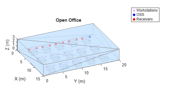

Use the supporting function iSimulateMeasurements to simulate the required measurements along the path. The function encapsulates the Simulate Measurements section.

measurements = iSimulateMeasurements(room,tx,rx,fs, ...
    L_poss1mff_base=L_poss1mff_base, ...
    L_poss1mff_jitter=L_poss1mff_jitter, ...
    decayPerDoubling=decayPerDoubling, ...
    ossSpatialJitter=ossSpatialJitter, ...
    L_pB_base=L_pB_base, ...
    L_pB_jitter=L_pB_jitter, ...
    rirNoiseFloor=noiseFloor);

Use the supporting function iComputeISO3382Metrics to compute the single-value quantities.

[r_D_path2,D_2S_path2,L_pAS4m_path2,r_C_path2,L_pB_path2] = iComputeISO3382Metrics(fs,measurements);

If you call the supporting function without output arguments, it plots the comfort and distraction distance for analysis.

iComputeISO3382Metrics(fs,measurements)

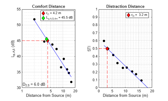
$Figure contains 2 axes objects. Axes object 1 with title Comfort Distance, xlabel Distance from Source (m), ylabel L_{p,A,S} (dB) contains 6 objects of type line. One or more of the lines displays its values using only markers These objects represent r_C = 4.2 m, L_{p,A,S,4m} = 45.5 dB. Axes object 2 with title Distraction Distance, xlabel Distance from Source (m), ylabel STI contains 5 objects of type line. One or more of the lines displays its values using only markers This object represents r_D = 3.2 m.$

ans = 
3.2042

Average the single-value metrics across the paths.

r_D_avg = mean([r_D,r_D_path2]);
D_2S_avg = mean([D_2S,D_2S_path2]);
L_pAS4m_avg = mean([L_pAS4m,L_pAS4m_path2]);
r_C_avg = mean([r_C,r_C_path2]);

Interpretation and Reporting

The ISO 3382-3:2020 standard provides a set of requirements for reporting, which include the single-number values to be reported for each acoustic zone in an open-plan office.

Calculate the average and standard deviation of the A-weighted SPL of background noise. For the average, calculate as the energy-mean of per-position A-weighted levels. For standard deviation, calculate the standard deviation of per-position A-weighted dB values.

L_pB_all = [L_pB;L_pB_path2];
L_pB_Ai = L_pB_all + Ai;
LpAB_Ai_pos_pow = sum(db2pow(L_pB_Ai),2);
LpAB_mean = pow2db(mean(LpAB_Ai_pos_pow));
LpAB_std = std(pow2db(LpAB_Ai_pos_pow));

Display a table as recommended in section 7 Test report of the standard (Table 2).

descriptions = [
    "Distraction distance in m";
    "Spatial decay rate of A-weighted SPL of speech in dB";
    "A-weighted SPL of speech at 4.0 meters in dB";
    "Comfort distance in m";
    "Average of A-weighted SPL of background noise in dB";
    "Standard deviation of A-weighted SPL of background noise in dB"
    ];
singleNumberValues = [r_D_avg,D_2S_avg,L_pAS4m_avg,r_C_avg,LpAB_mean,LpAB_std];

descWidth = 65;
valWidth = 10;

tableStr = "";
tableStr = tableStr + sprintf('+%s+%s+\n', repmat('-',1,descWidth+2), repmat('-',1,valWidth+2));
tableStr = tableStr + sprintf('| %-*s | %-*s |\n',descWidth,'Single-number quantity',valWidth,'Zone A');
tableStr = tableStr + sprintf('+%s+%s+\n',repmat('=',1,descWidth+2),repmat('=',1,valWidth+2));
for ii = 1:numel(singleNumberValues)
    tableStr = tableStr + sprintf('| %-*s | %*.1f |\n',descWidth,descriptions(ii),valWidth,singleNumberValues(ii));
end
tableStr = tableStr + sprintf('+%s+%s+\n',repmat('-',1,descWidth+2),repmat('-',1,valWidth+2));

fprintf('%s', tableStr);

+-------------------------------------------------------------------+------------+
| Single-number quantity                                            | Zone A     |
+===================================================================+============+
| Distraction distance in m                                         |        3.5 |
| Spatial decay rate of A-weighted SPL of speech in dB              |        6.2 |
| A-weighted SPL of speech at 4.0 meters in dB                      |       46.0 |
| Comfort distance in m                                             |        4.5 |
| Average of A-weighted SPL of background noise in dB               |       41.2 |
| Standard deviation of A-weighted SPL of background noise in dB    |        0.6 |
+-------------------------------------------------------------------+------------+

Annex C provides typical single-number values for poor and good room acoustics for a furnished open-plan office which is already in use.

Typical single-number values indicating poor room acoustic conditions are:

Distraction distance $r_{D} > 11$ m
Spatial decay rate of A-weighted SPL of speech $D_{2, S} < 5 dB$
A-weighted SPL of speech at 4.0 meters $L_{p, A, S, 4 m} > 52$ dB
Comfort distance $r_{C} > 11$ m
Average of A-weighted SPL of background noise $L_{p, A, B} < 35 or L_{p, A, B} > 48$

Typical single-number values indicating good room acoustic conditions are:

Distraction distance $r_{D} < 5$ m
Spatial decay rate of A-weighted SPL of speech $D_{2, S} > 8 dB$
A-weighted SPL of speech at 4.0 meters $L_{p, A, S, 4 m} > 42 dB$
Comfort distance $r_{C} < 5$
Average of A-weighted SPL of background noise $L_{p, A, B}$ within $40 dB$ to $45 dB$

Supporting Functions

Add Noise Floor

function ir = iAddNoiseFloor(ir,fs,noiseFloor)
% Minimum duration for IR captures for ISO 3382 compliance
flength = ceil(1.6*fs);

% Zero-pad IR to minimum length
if size(ir,2) < flength
    ir = resize(ir,flength,Dimension=2);
end

% Generate pink noise and normalize rms.
noise = pinknoise(size(ir,2),size(ir,1));
noise = noise./rms(noise);

% Scale pink noise to desired rms.
noise_rms = max(abs(ir),[],2) * 10^(noiseFloor/20);
noise = noise.*noise_rms';

ir = ir + noise';
end

Create Room

function [TR,workstationLocations] = iCreateRoom(roomDimensions)
arguments
    roomDimensions = []
end
figure()

L = roomDimensions(1);
W = roomDimensions(2);
H = roomDimensions(3);

% Room vertices and faces (triangles)
roomVerts = [
    0 0 0;      % 1
    L 0 0;      % 2
    L W 0;      % 3
    0 W 0;      % 4
    0 0 H;      % 5
    L 0 H;      % 6
    L W H;      % 7
    0 W H];     % 8

% Two triangles per face (12 total)
roomFaces = [
    1 2 3; 1 3 4;    % bottom
    5 6 7; 5 7 8;    % top
    1 2 6; 1 6 5;    % front
    2 3 7; 2 7 6;    % right
    3 4 8; 3 8 7;    % back
    4 1 5; 4 5 8];   % left

allVerts = roomVerts;
allFaces = roomFaces;

% Table parameters and positions
tableLength = 2;   % along X (meters)
tableWidth  = 1.5; % along Y (meters)
tableHeight = 0.8; % along Z (meters)
nRows = 5;
nCols = 3;
rowSpacing = 2; % space between rows (Y direction)
colSpacing = 3; % space between columns (X direction)
xOffset = 2;    % margin from left wall
yOffset = 2;    % margin from front wall

headHeight = 1.2;
edgeMargin = 0.25;
workstationLocations = [];

for row = 1:nRows
    for col = 1:nCols
        x0 = xOffset + (col-1)*(tableLength+colSpacing);
        y0 = yOffset + (row-1)*(tableWidth+rowSpacing);
        z0 = 0; % tables sit on floor

        % Make sure tables fit in the room
        [vTab, fTab] = iCreateTable(x0, y0, z0, tableLength, tableWidth, tableHeight);

        % Adjust face indices to global vertex list
        idxOffset = size(allVerts,1);
        fTab = fTab + idxOffset;

        % Add to overall lists
        allVerts = [allVerts; vTab]; %#ok<*AGROW>
        allFaces = [allFaces; fTab];

        % Add two workstation locations per table, centered in X, one on each side in Y
        cx = x0 + tableLength/2;
        ws1 = [cx, y0 - edgeMargin, headHeight];              % front side
        ws2 = [cx, y0 + tableWidth + edgeMargin, headHeight]; % back side
        workstationLocations = [workstationLocations; ws1; ws2];
    end
end

% Create the global triangulation object
TR = triangulation(allFaces, allVerts);

    function [verts, faces] = iCreateTable(x, y, z, l, w, h)
        % Returns 8 vertices and 12 faces (triangles) for a cuboid table
        verts = [
            x    y    z;      % 1
            x+l  y    z;      % 2
            x+l  y+w  z;      % 3
            x    y+w  z;      % 4
            x    y    z+h;    % 5
            x+l  y    z+h;    % 6
            x+l  y+w  z+h;    % 7
            x    y+w  z+h];   % 8

        faces = [
            1 2 3; 1 3 4;    % bottom
            5 6 7; 5 7 8;    % top
            1 2 6; 1 6 5;    % front
            2 3 7; 2 7 6;    % right
            3 4 8; 3 8 7;    % back
            4 1 5; 4 5 8];   % left
    end
end

Plot Room

function iPlotRoom(room,wsLocs,sourceCoord,receiverCoord)
arguments
    room
    wsLocs = []
    sourceCoord = []
    receiverCoord = []
end
figure()

trisurf(room, ...
    FaceColor=[0.8 0.9 1], ...
    FaceAlpha=0.7, ...
    EdgeColor=[0.5 0.5 0.5]);
hold on

if ~isempty(wsLocs)
    wp = plot3(wsLocs(:,1),wsLocs(:,2),wsLocs(:,3), "om",MarkerSize=3,LineWidth=0.5,MarkerFaceColor="none");
end
if ~isempty(sourceCoord)
    sp = plot3(sourceCoord(1),sourceCoord(2),sourceCoord(3),"ob",MarkerSize=4,LineWidth=2,MarkerFaceColor="b");
    rp = plot3(receiverCoord(:,1),receiverCoord(:,2),receiverCoord(:,3),"or",MarkerSize=4,LineWidth=2,MarkerFaceColor="r");
end
if ~isempty(sourceCoord)
    legend([wp,sp,rp],"Workstations","OSS","Receivers")
else
    legend(wp,"Workstations")
end

xlabel("X (m)")
ylabel("Y (m)")
zlabel("Z (m)")
grid on
axis equal
title("Open Office")
view([65.12 26.91])
hold off
end

Simulate Measurements

function measurements = iSimulateMeasurements(room,tx,rx,fs,options)
arguments
    room
    tx (1,3) double
    rx (:,3) double
    fs (1,1) double
    options.L_poss1mff_base (1,7) double = 80*ones(1,7)
    options.L_poss1mff_jitter (1,1) double = 4
    options.decayPerDoubling (1,1) double = 5
    options.ossSpatialJitter (1,1) double = 6
    options.L_pB_base (1,7) double = [44 41 38 35 32 29 26]
    options.L_pB_jitter (1,1) double = 6
    options.rirNoiseFloor (1,1) double = -60
end

bands = [125 250 500 1000 2000 4000 8000];

% Distances (straight line)
r_n = vecnorm(rx - tx,2,2);

% Simulate OSS 1 m free-field spectrum with jitter
L_poss1mff = options.L_poss1mff_base + (options.L_poss1mff_jitter*(rand(1,7)-0.5));

% Build L_p,tot per receiver using a simple distance law and spatial variability
d0 = 1;
N = size(rx,1);
spatialJitter = options.ossSpatialJitter*(rand(N,7) - 0.5); % +/- half range
L_ptot = L_poss1mff - options.decayPerDoubling*log2(r_n./d0) + spatialJitter;

% Background noise per receiver
L_pB = options.L_pB_base + (options.L_pB_jitter*(rand(N,7) - 0.5));

% Simulate RIRs and add noise floor
rir = acousticRoomResponse(room, tx, rx, SampleRate=fs);
rir = iAddNoiseFloor(rir, fs, options.rirNoiseFloor);

% Package
measurements = struct(SampleRate=fs, ...
    bands=bands, ... Octave band centers (Hz)
    r_n=r_n(:), ... Distance from OSS to receiver on path (m)
    L_poss1mff=L_poss1mff, ... Measured SPL of OSS at 1 meter in a free field
    L_ptot=L_ptot, ... Measured SPL includes both OSS and background noise
    L_pB=L_pB, ... Measured background noise SPL (OSS is off)
    rir=rir); % Measured RIR at each receiver from OSS location as transmitter
end

Compute ISO 3382-3 Metrics

function [r_D,D_2S,L_pAS4m,r_C,L_pB] = iComputeISO3382Metrics(fs,measurements)
arguments
    fs (1,1) double
    measurements struct
end

r_n = measurements.r_n;
L_poss1mff = measurements.L_poss1mff;
L_ptot = measurements.L_ptot;
L_pB = measurements.L_pB;
rir = measurements.rir;
Ai = [-16.1 -8.6 -3.2 0 1.2 1.0 -1.1];
L_pS1mff = [49.9 54.3 58.0 52.0 44.8 38.8 33.5];

% Background-noise correction octave by octave
L_poss = pow2db( max( db2pow(L_ptot) - db2pow(L_pB), eps) );

% Attenuation
D_ni = L_poss1mff - L_poss;

% Map to normal speech
L_pSni = L_pS1mff - D_ni;

% A-weighted overall speech per position
L_pASn = pow2db( sum( db2pow(L_pSni + Ai), 2 ) );

% Fit D2,S over distances 2–16 m
fitMask = (r_n >= 2) & (r_n <= 16);
r_fit = r_n(fitMask);
L_fit = L_pASn(fitMask);
r0 = 1;
N = numel(r_fit);
x = log10(r_fit/r0);
num = N*sum(L_fit.*x) - sum(L_fit)*sum(x);
den = N*sum(x.^2) - (sum(x))^2;
D_2S = -log10(2)*(num/den);

% L_p,A,S,4m
L_pAS4m = mean(L_fit) + D_2S * mean( log2(r_fit/4) );

% Comfort distance r_C (Formula 8)
r_C = 2.^((L_pAS4m - 45 + 2*D_2S)/D_2S);

% STI per position using average L_p,B along the path (standard guidance)
L_pB_avg = mean(L_pB,1);
sti = nan(size(r_n));
for ii = 1:size(rir,1)
    sti(ii) = speechTransmissionIndex(rir(ii,:), fs, ...
        OperationalSignalLevel = L_pSni(ii,:), ...
        OperationalNoiseLevel  = L_pB_avg);
end

% Linear fit STI vs distance
sti_fit = polyfit(r_n, sti, 1);
yfit_sti = polyval(sti_fit, [r_n;20]);
r_D = (0.50 - sti_fit(2)) / sti_fit(1);

if nargout==0

    figure
    tiledlayout(1,2)
    
    nexttile()

    semilogx(r_n,L_pASn,"ok",MarkerFaceColor="k",MarkerSize=5);
    hold on
    xlabel("Distance from Source (m)")
    ylabel("L_{p,A,S} (dB)")

    grid on
    grid minor

    xlim([1,20])
    xticks([1,5,10,20])

    % Plot fit line
    fitmask = r_n >= 2 & r_n <= 16;
    L_pASn_masked = L_pASn(fitmask);
    r_n_masked = r_n(fitmask);
    x = log2(r_n_masked/r0);
    a = mean(L_pASn_masked) + D_2S * mean(x);
    yfit = a - D_2S*log2(r_n_masked/r0);
    plot(r_n_masked,yfit,"b-",LineWidth=0.1)

    % Plot comfort distance threshold (45 dB)
    plot([1,r_C],[45 45],"--r",LineWidth=0.1)
    plot([r_C,r_C],[30 45],"--r",LineWidth=0.1)

    % Mark comfort distance
    h1 = plot(r_C,45,"dk",MarkerFaceColor="r",MarkerSize=7);
    h2 = plot(4,L_pAS4m,"dk",MarkerFaceColor="g",MarkerSize=7);

    title("Comfort Distance")

    annotation("textbox",[0.12,0.1,0.2,0.1],String=sprintf('D_{2,S} = %0.1f dB',D_2S),EdgeColor="none")

    legend([h1,h2],sprintf('r_C = %0.1f m',r_C),sprintf('L_{p,A,S,4m} = %0.1f dB',L_pAS4m),Location="best")
    hold off

    nexttile

    plot(r_n,sti,"ok",MarkerFaceColor="k",MarkerSize=5)

    grid on
    grid minor
    xlabel("Distance from Source (m)")
    ylabel("STI")
    hold on
    plot([r_n;20],yfit_sti,"b-")
    plot([0;r_D],[0.5,0.5],"--r",LineWidth=0.1)
    plot([r_D;r_D],[0,0.5],"--r",LineWidth=0.1)
    title("Distraction Distance")

    h = plot(r_D,0.5,"dk",MarkerFaceColor="r",MarkerSize=7);

    ylim([0,1])

    legend(h,sprintf("r_D =  %0.1f m",r_D))
    hold off
end
end

References

[1] ISO 3382-3:2022. "Acoustics — Measurement of room acoustic parameters — Part 3: Open plan offices." International Organization for Standardization.

Comfort Distance and Distraction Distance (ISO 3382-3)

Model Room

Simulate Measurements

Spatial Decay Rate of Speech

Comfort Distance

Distraction Distance

Measure Multiple Paths

Interpretation and Reporting

Supporting Functions

Add Noise Floor

Create Room

Plot Room

Simulate Measurements

Compute ISO 3382-3 Metrics

References

See Also