Eye Diagram
(Removed) Display eye diagram of time-domain signal
In R2025a, eye diagram analysis, such as measurements, histograms, and bathtub curves, has been removed from the Eye Diagram block. For more information, see Version History
Libraries:
Communications Toolbox /
Comm Sinks
Communications Toolbox HDL Support /
Comm Sinks
Mixed-Signal Blockset /
Utilities
SerDes Toolbox /
Utilities
Description
The Eye Diagram block displays multiple traces of a modulated signal to produce an eye diagram. You can use the block to reveal the modulation characteristics of the signal, such as the effects of pulse shaping or channel distortions.
The Eye Diagram block has one input port. This block accepts a column vector or scalar input signal. The block accepts a signal with the following data types: double, single, base integer, and fixed point. All data types are cast as double before the block displays results.
To modify the eye diagram display, select View > Configuration Properties or click the Configuration Properties button (![]() ). Then select the Main, 2D color
histogram, Axes, or Export tabs
and modify the settings.
). Then select the Main, 2D color
histogram, Axes, or Export tabs
and modify the settings.

Ports
Input
Input signal, specified as a scalar or column vector.
Data Types: double
Parameters
Main Tab
Display mode of the eye diagram, specified as Line
plot or 2D color histogram.
Selecting 2D color histogram makes the
histogram tab available.
Tunable: Yes
Select this check box to enable eye measurements of the input signal.
Select this radio button to display the jitter histogram. This can also be accessed by using the histogram button drop down on the toolbar.
Dependencies
This parameter is available when Display mode
is 2D color histogram and
Enable measurements is selected.
Select this radio button to display the noise histogram. This can also be accessed by using the histogram button drop down on the toolbar.
Dependencies
This parameter is available when Display mode
is 2D color histogram and
Enable measurements is selected.
Select this radio button to display neither the histogram noise nor the histogram jitter.
Dependencies
This parameter is available when Display mode
is 2D color histogram and
Enable measurements is selected.
Select this check box to display the horizontal bathtub curve. This can also be accessed by using the bathtub curve button on the toolbar.
Dependencies
This parameter is available when Enable measurements is selected.
Select this check box to display the vertical bathtub curve. This can also be accessed by using the bathtub curve button on the toolbar.
Dependencies
This parameter is available when Enable measurements is selected.
Select either Real only or
Real and imaginary to display one or both
eye diagrams. To make eye measurements, this parameter must be
Real only.
Tunable: Yes
Select this check box to fade the points in the display as the interval of time after they are first plotted increases.
Tunable: Yes
Dependencies
This parameter is available only when the Display
mode is Line plot.
Number of samples per symbol, specified as a positive integer. Use with Symbols per trace to determine the number of samples per trace.
Tunable: Yes
Sample offset, specified as a nonnegative integer smaller than the product of Samples per symbol and Symbols per trace. The offset provides the number of samples to omit before plotting the first point.
Tunable: Yes
Number of symbols plotted per trace, specified as a positive integer.
Tunable: Yes
Number of traces plotted, specified as a positive integer.
Tunable: Yes
Dependencies
This parameter is available only when the Display
mode is Line plot
Axes Tab
Label that appears above the eye diagram plot.
Tunable: Yes
Toggle this check box to turn the grid on and off.
Tunable: Yes
Minimum value of the y-axis.
Tunable: Yes
Maximum value of the y-axis.
Tunable: Yes
Text that the scope displays along the real axis.
Tunable: Yes
Text that the scope displays along the imaginary axis.
Tunable: Yes
2D Histogram Tab
The 2D histogram tab is available when you click the histogram button or when the
display mode is set to 2D color histogram.
Oversampling method, specified as None,
Input interpolation, or
Histogram interpolation.
To plot eye diagrams as quickly as possible, set the
Oversampling method to
None. The drawback to not oversampling is
that the plots look pixelated when the number of samples per trace is
small. To create smoother, less-pixelated plots using a small number of
samples per trace, set the Oversampling method to
Input interpolation or
Histogram interpolation.
Input interpolation is the faster of the
two interpolation methods and produces good results when the
signal-to-noise ratio (SNR) is high. With a lower SNR, this oversampling
method is not recommended because it introduces a bias to the centers of
the histogram ranges. Histogram interpolation
is not as fast as the other techniques, but it provides good results
even when the SNR is low.
Tunable: Yes
Color scale of the histogram plot, specified as either
Linear or
Logarithmic. Set Color
scale to Logarithmic if
certain areas of the eye diagram include a disproportionate number of
points.
Tunable: Yes
The toolbar contains a histogram reset button ![]() , which resets the internal histogram buffers and clears the
display. This button is not available when the display mode is set to
, which resets the internal histogram buffers and clears the
display. This button is not available when the display mode is set to
Line plot.
Export Tab
Select this check box export the eye diagram measurements to the MATLAB® workspace.
Tunable: Yes
Specify the name of the variable to which the eye diagram measurements are saved. The data is saved as a structure having these fields:
MeasurementSettingsMeasurementsJitterHistogramNoiseHistogramHorizontalBathtubVerticalBathtubBlockName
Tunable: Yes
Style Dialog Box
In the Style dialog box, you can customize the style of the active display. You can change the color of the figure containing the displays, the background and foreground colors of display axes, and properties of lines in a display. To open this dialog box, select View > Style.
Specify the background color of the scope figure.
Specify the fill and line colors for the axes.
Specify the line style, line width, and line color for the displayed signal.
Dependencies
This parameter is available only when the Display
mode is Line plot.
Data point marker for the selected signal, specified as one of the
choices in this table data point markers. This parameter is similar to
the Marker property for MATLAB
Handle Graphics® plot objects.
| Specifier | Marker Type |
|---|---|
| none | No marker (default) |
|
| Circle |
|
| Square |
|
| Cross |
|
| Point |
|
| Plus sign |
|
| Asterisk |
|
| Diamond |
|
| Downward-pointing triangle |
|
| Upward-pointing triangle |
|
| Left-pointing triangle |
|
| Right-pointing triangle |
|
| Five-pointed star (pentagram) |
|
| Six-pointed star (hexagram) |
Dependencies
This parameter is available only when the Display
mode is Line plot.
Specify the colormap of the histogram plots as one of these schemes:
Parula, Jet,
HSV, Hot,
Cool, Spring,
Summer,
Autumn, Winter,
Gray, Bone,
Copper, Pink,
Lines, or
Custom. If you select
Custom, a dialog box pops up from which you can
enter code to specify your own colormap.
Dependencies
This parameter is available only when the Display
mode is 2D color
histogram.
Measurement Settings Pane
To change measurement settings, first select Enable measurements. Then, in the Eye Measurements pane, click the arrow next to Settings. You can control these measurement settings.
Time range for calculating eye levels, specified as a two-element vector. These values are expressed as a percentage of the symbol duration.
Tunable: Yes
Amplitude level threshold in V, specified as a scalar. This parameter separates the different signaling regions for horizontal (jitter) histograms. This parameter is tunable, but the jitter histograms reset when the parameter changes.
For non-return-to-zero (NRZ) signals, set Decision boundary to 0. For return-to-zero (RZ) signals, set Decision boundary to half the maximum amplitude.
Tunable: Yes
Amplitude levels of the rise and fall transitions, specified as a two-element vector. These values are expressed as a percentage of the eye amplitude. This parameter is tunable, but the crossing histograms of the rise and fall thresholds reset when the parameter changes.
Tunable: Yes
Amplitude tolerance of the horizontal crossings in V, specified as a scalar. Increase hysteresis to provide more tolerance to spurious crossings due to noise. This parameter is tunable, but the jitter and the rise and fall histograms reset when the parameter changes.
Tunable: Yes
BER used for eye measurements, specified as a nonnegative scalar from 0 to 0.5. The value is used to make measurements of random jitter, total jitter, horizontal eye openings, and vertical eye openings.
Tunable: Yes
BER values used to calculate openings of bathtub curves, specified as a vector whose elements range from 0 to 0.5. Horizontal and vertical eye openings are calculated for each of the values specified by this parameter.
Tunable: Yes
Dependencies
To enable this parameter, select Show horizontal bathtub curve, Show vertical bathtub curve, or both.
Duration of initial data discarded from measurements, in seconds, specified as a nonnegative scalar.
Block Characteristics
Data Types |
|
Direct Feedthrough |
|
Multidimensional Signals |
|
Variable-Size Signals |
|
Zero-Crossing Detection |
|
More About
When an Eye Diagram block is placed in a conditionally executed subsystem, for example in a triggered or enabled subsystem:
Input size must be an integer multiple of
SamplesPerSymbol*SymbolsPerTraceSample offset must be zero
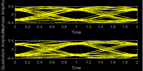
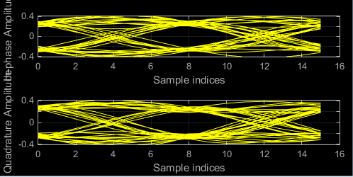
The rightmost part of the display is intentionally omitted. This figure compares typical eye diagram display when placed in a normal system versus one placed in a conditionally executed subsystem.
Eye Diagram Plot in Normal System Eye Diagram Plot in Conditionally Executed Subsystem 

In a regular Eye Diagram, the rightmost part is a line between the last sample of a trace and the first sample of the next trace. In conditionally executed subsystems, these traces may be non-contiguous, thus this rightmost segment could corrupt the display and is omitted.
Measurements assume that the eye diagram object has valid data. A valid eye diagram has two distinct eye crossing points and two distinct eye levels.
To open the measurements pane, click on the Eye Measurements button or select Tools > Measurements > Eye Measurements from the toolbar menu.
Note
For amplitude measurements, at least one bin per vertical histogram must reach 10 hits before the measurement is taken, ensuring higher accuracy.
For time measurements, at least one bin per horizontal histogram must reach 10 hits before the measurement is taken.
When an eye crossing time measurement falls within the [-0.5/Fs, 0) seconds interval, the time measurement wraps to the end of the eye diagram, i.e., the measurement wraps by 2×Ts seconds (where Ts is the symbol time). For a complex signal case, the analyze method issues a warning if the crossing time measurement of the in-phase branch wraps while that of the quadrature branch does not (or vice versa). To avoid time-wrapping or a warning, add a half-symbol duration delay to the current value in the
MeasurementDelayproperty of the eye diagram object. This additional delay repositions the eye in the approximate center of the scope.
- Eye Levels - Amplitude level used to represent data bits
Eye level is the amplitude level used to represent data bits. For the displayed NRZ signal, the levels are –1 V and +1 V. The eye levels are calculated by averaging the 2-D histogram within the eye level boundaries. For example, when the
EyeLevelBoundariesproperty is set to[40 60], that is, 40% and 60% of the symbol duration, the eye levels are calculated by estimating the mean value of the vertical histogram in this window marked by the eye level boundaries.
- Eye Amplitude - Distance between eye levels
Eye amplitude is the distance in V between the mean value of two eye levels.

- Eye Height - Statistical minimum distance between eye levels
Eye height is the distance between μ – 3σ of the upper eye level and μ + 3σ of the lower eye level. μ is the mean of the eye level, and σ is the standard deviation.

- Vertical Opening - Distance between BER threshold points
The vertical opening is the distance between the two points that correspond to the
BERThresholdproperty. For example, for a BER threshold of 10–12, these points correspond to the 7σ distance from each eye level.
- Eye SNR - Signal-to-noise ratio
The eye SNR is the ratio of the eye level difference to the difference of the vertical standard deviations corresponding to each eye level:
where L1 and L0 represent the means of the upper and lower eye levels and σ1 and σ0 represent their standard deviations.
- Q Factor - Quality factor
The Q factor is the quality factor and is calculated using the same formula as the eye SNR. However, the standard deviations of the vertical histograms are replaced with those computed with the dual-Dirac analysis.
- Crossing Levels - Amplitude levels for eye crossings
The crossing levels are the amplitude levels at which the eye crossings occur.
The level at which the input signal crosses the amplitude value is specified by the
DecisionBoundaryproperty.
- Crossing Times - Times for which crossings occur
The crossing times are the times at which the crossings occur. The times are computed as the mean values of the horizontal (jitter) histograms.

- Eye Delay - Mean time between eye crossings
Eye delay is the midpoint between the two crossing times.

- Eye Width - Statistical minimum time between eye crossings
Eye width is the horizontal distance between μ + 3σ of the left crossing time and μ – 3σ of the right crossing time. μ is the mean of the jitter histogram, and σ is the standard deviation.

- Horizontal Opening - Time between BER threshold points
The horizontal opening is the distance between the two points that correspond to the
BERThresholdproperty. For example, for a 10–12 BER, these two points correspond to the 7σ distance from each crossing time.
- Rise Time - Time to transition from low to high
Rise time is the mean time between the low and high rise/fall thresholds defined in the eye diagram. The default thresholds are 10% and 90% of the eye amplitude.

- Fall Time - Time to transition from high to low
Fall time is the mean time between the high and low rise/fall thresholds defined in the eye diagram. The default thresholds are 10% and 90% of the eye amplitude.

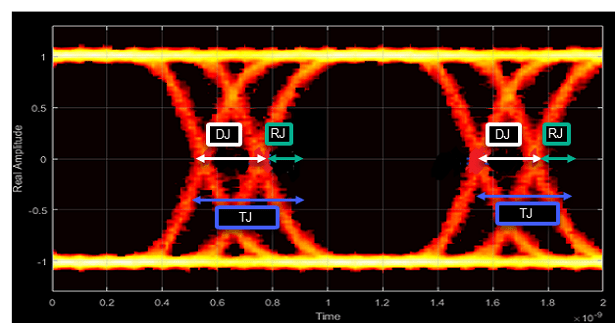
- Deterministic Jitter - Deterministic deviation from ideal signal timing
Jitter is the deviation of a signal’s timing event from its intended (ideal) occurrence in time [2]. Jitter can be represented with a dual-Dirac model. A dual-Dirac model assumes that the jitter has two components: deterministic jitter (DJ) and random jitter (RJ).
DJ is the distance between the two peaks of the dual-Dirac histograms. The probability density function (PDF) of DJ is composed of two delta functions.

- Random Jitter - Random deviation from ideal signal timing
RJ is the Gaussian unbounded jitter component. The random component of jitter is modeled as a zero-mean Gaussian random variable with a specified standard-deviation of σ. The RJ is computed as:
where
BER is the specified BER threshold. ρ is the amplitude of the left and right Dirac function, which is determined from the bin counts of the jitter histograms.

- Total Jitter - Deviation from ideal signal timing
Total jitter (TJ) is the sum of the deterministic and random jitter, such that TJ = DJ + RJ.

The total jitter PDF is the convolution of the DJ PDF and the RJ PDF.

- RMS Jitter - Standard deviation of jitter
RMS jitter is the standard deviation of the jitter calculated in the horizontal (jitter) histogram at the decision boundary.

- Peak-to-Peak Jitter - Distance between extreme data points of histogram
Peak-to-peak jitter is the maximum horizontal distance between the left and right nonzero values in the horizontal histogram of each crossing time.

Display the eye diagram of a filtered QPSK signal using the Eye Diagram block.
Build the
doc_eye_diagram_scope model as shown in this figure.

Run the model and observe that two symbols are displayed.

Open the configuration parameters dialog box. Change the Symbols per trace parameter to 4. Run the simulation and observe that four symbols are displayed.

Try changing the Raised Cosine Transmit Filter parameters or changing additional Eye Diagram parameters to see their effects on the eye diagram.
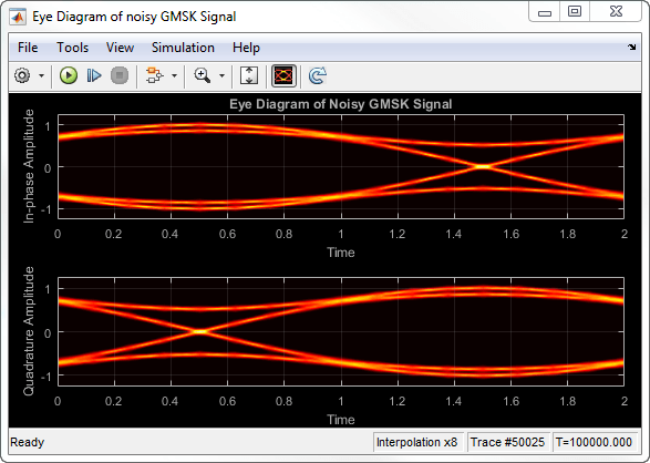
Display histogram plots of a noisy GMSK signal.
Build the
doc_eye_diagram_gmsk model as shown in this
figure.

Run the model. The eye diagram is configured to show a histogram without interpolation.

The lack of interpolation results in a plot having piecewise-continuous behavior.
Open the 2D Histogram tab of the Configuration
Properties dialog box. Set the Oversampling method to
Input interpolation. Run the model.

The interpolation smooths the eye diagram.
On the AWGN Channel block, change SNR
(dB) from 25 to 10. Run
the model.

Observe that vertical striping is present in the eye diagram. This striping is the result of input interpolation, which has limited accuracy in low-SNR conditions.
Set the Oversampling method to Histogram
interpolation. Run the model.

The eye diagram plot now renders accurately because the histogram interpolation method works for all SNR values. This method is not as fast as the other techniques and results in increased execution time.
You can programmatically configure the scope properties with callbacks or within scripts by using a scope configuration object as describe in Control Scope Blocks Programmatically (Simulink).
Extended Capabilities
This block is excluded from the generated code when code generation is performed on a system containing this block.
This block can be used for simulation visibility in subsystems that generate HDL code, but is not included in the hardware implementation.
Version History
Introduced in R2014aEye diagram analysis, such as measurements, histograms, and bathtub curves, have be removed from the Eye Diagram block. To access these functionalities you need licenses to Signal Integrity Toolbox™, SerDes Toolbox™, or Mixed-Signal Blockset™.
Use the
eyeDiagramSI(Signal Integrity Toolbox) system object, Eye Measurement (Signal Integrity Toolbox) block,eyeContour(Signal Integrity Toolbox) object, andeyeMask(Signal Integrity Toolbox)object to measure eye diagram metrics such as eye height, width, area, linearity, vertical eye closure (VEC), and channel operating margin (COM).For the new eye diagram block in Communications Toolbox™, see Eye Diagram.
Eye diagram analysis, such as measurements, histograms, and bathtub curves, will be removed from the Eye Diagram block in a future release. To access these functionalities:
Refer to Measurements and Testbenches (Mixed-Signal Blockset) to analyze performance metrics such as phase noise, reference and fractional spurs, aperture jitter, timing impairments, and lock time.
Refer to Get Started with SerDes Toolbox (SerDes Toolbox) export a Simulink model and assess metrics such as bathtub curve and channel operating margin (COM), including the effects of jitter and crosstalk.
Refer to Analyze Serial Links with Serial Link Designer (Signal Integrity Toolbox) and Analyze Parallel Links with Parallel Link Designer (Signal Integrity Toolbox) to understand how to set up a topology or use one of the predefined ‘kits’ to run simulations of interest. Use the Signal Integrity Viewer app to view the waveforms, bathtubs, measurements, and more.
For the new eye diagram block, see Eye Diagram.
MATLAB Command
You clicked a link that corresponds to this MATLAB command:
Run the command by entering it in the MATLAB Command Window. Web browsers do not support MATLAB commands.
Sélectionner un site web
Choisissez un site web pour accéder au contenu traduit dans votre langue (lorsqu'il est disponible) et voir les événements et les offres locales. D’après votre position, nous vous recommandons de sélectionner la région suivante : .
Vous pouvez également sélectionner un site web dans la liste suivante :
Comment optimiser les performances du site
Pour optimiser les performances du site, sélectionnez la région Chine (en chinois ou en anglais). Les sites de MathWorks pour les autres pays ne sont pas optimisés pour les visites provenant de votre région.
Amériques
- América Latina (Español)
- Canada (English)
- United States (English)
Europe
- Belgium (English)
- Denmark (English)
- Deutschland (Deutsch)
- España (Español)
- Finland (English)
- France (Français)
- Ireland (English)
- Italia (Italiano)
- Luxembourg (English)
- Netherlands (English)
- Norway (English)
- Österreich (Deutsch)
- Portugal (English)
- Sweden (English)
- Switzerland
- United Kingdom (English)