Assemble Parts of System Using Coupling Interfaces
This example shows how to model a mass-spring-damper system using physical assembly of individual components. You use addInterface and assemble to model this system as individual components and interface coupling forces separately for each component. This is helpful when you have individual components and want to assemble them with other parts by defining an internal coupling.
Physical Coupling Overview
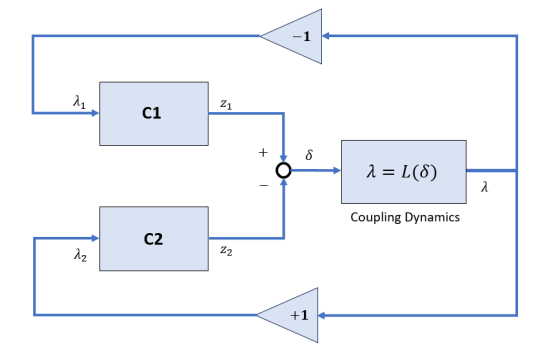
In generalized coordinates, you can specify couplings as additional inputs and outputs of the system.
In general, you can represent physical couplings in a block diagram form as shown in the following figure. The coupling is characterized by the "Coupling Dynamics" block mapping (collocation gap) to the internal forces . Here, and denote the positions on each part of the nodes being coupled together.
Using Control System Toolbox™, you can perform the following types of couplings between state-space models.
Rigid couplings, which correspond to and determined by the balance of forces. In this type of coupling, the positions, and match exactly (collocation) as if the two parts were welded together.
Compliant couplings, where . Here the coupling is modeled as a spring-damper connection and the two parts can move with respect to each other.
Generalized coupling, where . Here, you obtain as the output of a linear system driven by the gap . This can be used to model more complex coupling dynamics.
For more information, see the Algorithms section on the assemble reference page.
Modeling Mass-Spring-Damper Dynamics
For this example, consider a mass-spring-damper system where two masses are connected by a spring and damper and the second mass is connected to a wall with another spring and damper, with an external force acting on mass 1. Mass 1 exerts a force on mass 2, while mass 2 exerts the force on mass 1. Similarly, mass 2 exerts a coupling force on the wall and gets in return.
Here, and are the masses, and and are the displacements of mass 1 and 2, respectively. Additionally, you define and as internal coupling forces using the addInterface function.
Define the model parameters.
m1 = 1.5; % kg
m2 = 2;   % kg
k1 = 10;  % N/m (between masses)
c1 = 1;   % Ns/m (between masses)
k2 = 20;  % N/m (mass 2 to wall)
c2 = 2;   % Ns/m (mass 2 to wall)
Define the dynamics of mass 1 in the state-space form.
Create the state-space model without the coupling force , as you will use addInterface to add that term in the next section.
A = [0 1; 0 0];
B = [0;1/m1];
C = [1 0];
sys1 = ss(A,B,C,0);
Similarly define the dynamics for the second mass.
Create the state-space model.
A2 = [0 1; 0 0];
B2 = [0;0]; % no external forces
C2 = [1 0];
sys2 = ss(A2,B2,C2,0);
Compliant Coupling
When you assemble parts using compliant coupling, the software models the coupling dynamics as , where is obtained as the output of linear system driven by the gap . Therefore, coupling between the two masses is defined as , as they are driven by the gap in displacement . And, the coupling between mass 2 and wall is defined as , which depends on the displacement from mass 2 as there is no displacement from the wall side.
Define the interface using addInterface.
Hu = [0; 1/m1];
Hy = [1 0]; % z1 = x1
sys1.Name = "m1";
sys1.InputName = "force";
sys1.OutputName = "x1";
sys1 = addInterface(sys1,"m1tom2",Hy,Hu);
Similarly, define the coupling interface at mass 2.
Hu2 = [0; 1/m2];
Hy2 = [1 0]; % z2 = x2
sys2.Name = "m2";
sys2.OutputName = "x2";
sys2 = addInterface(sys2,"m2tom1",Hy2,Hu2);
Finally, add the interface for the connection between m2 and wall.
sys2 = addInterface(sys2,"m2toW",Hy2,Hu2);Create the uncoupled superstructure using append.
sys = append(sys1,sys2);
Create the coupling between the two masses.
asys = assemble(sys,"m1:m1tom2","m2:m2tom1",k1,c1);
Create the coupling between the second mass and wall.
asys2 = assemble(asys,"m2:m2toW","Ground",k2,c2);
Compare Assembled Model with Complete Dynamics Model
You can define the mass-spring-damper model that accounts for complete dynamics from spring and damper couplings as follows.
Or, in the state-space form:
Create the state-space model.
Ac = [ 0, 1, 0, 0;
-k1/m1, -c1/m1, k1/m1, c1/m1;
0, 0, 0, 1;
k1/m2, c1/m2, -(k1+k2)/m2, -(c1+c2)/m2 ];
Bc = [ 0;
1/m1;
0;
0 ];
Cc = [1 0 0 0;
0 0 1 0]; % output x1 and x2
Dc = 0;
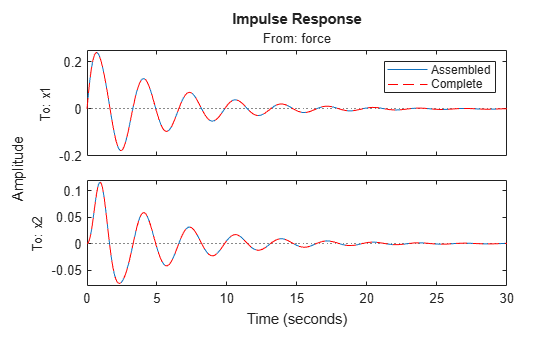
sysc = ss(Ac, Bc, Cc, Dc);Simulating the impulse response, you can see both models are equivalent.
impulseplot(asys2(:,1),sysc,"r--")
legend("Assembled","Complete")
Rigid Coupling
Suppose, you coupled both masses rigidly. In this type of coupling, the positions, and of the masses match exactly as if the two masses were welded together. This corresponds to a system with a single mass with value m1+m2, connected to a wall.
Create the rigid coupling between the two masses.
asys3 = assemble(sys,"m1:m1tom2","m2:m2tom1");
Create the compliant coupling to the wall.
asys3 = assemble(asys3,"m2:m2toW","Ground",k2,c2);
Additionally, define the model with complete dynamics for comparison.
m = m1+m2;
Ac = [0 1; -k2/m -c2/m];
Bc = [0;1/m];
Cc = [1 0];
Dc = 0;
sysc2 = ss(Ac,Bc,Cc,Dc);
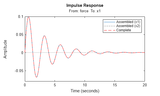
Simulating the impulse response, you can see both models are equivalent. While the assembled model asys3 contains two outputs and , you can see that they are both equal because the masses are rigidly coupled.
impulseplot(asys3(1,1),asys3(2,1),"k:",sysc2,"r--")
legend("Assembled (x1)","Assembled (x2)","Complete")