Specifying Time Delays
This example shows how the Control System Toolbox™ lets you represent, manipulate, and analyze any LTI model with a finite number of delays. The delays can be at the system inputs or outputs, between specific I/O pairs, or internal to the model (for example, inside a feedback loop).
Time Delays in LTI Models
Transfer function (TF), zero-pole-gain (ZPK), and frequency response data (FRD) objects offer three properties for modeling delays:
InputDelay, to specify delays at the inputs
OutputDelay, to specify delays at the outputs
IODelay, to specify independent transport delays for each I/O pair.
The state-space (SS) object has three delay-related properties as well:
InputDelay, to specify delays at the inputs
OutputDelay, to specify delays at the outputs
InternalDelay, to keep track of delays when combining models or closing feedback loops.
The ability to keep track of internal delays makes the state-space representation best suited to modeling and analyzing delay effects in control systems. This tutorial shows how to construct and manipulate systems with delays. For more information on how to analyze delay effects, see Analyze Control Systems with Delays.
First-Order Plus Dead Time Models
First-order plus dead time models are commonly used in process control applications. One such example is:

To specify this transfer function, use
num = 5;
den = [1 1];
P = tf(num,den,'InputDelay',3.4)
P =

                  5
  exp(-3.4*s) * -----
                s + 1

Continuous-time transfer function.
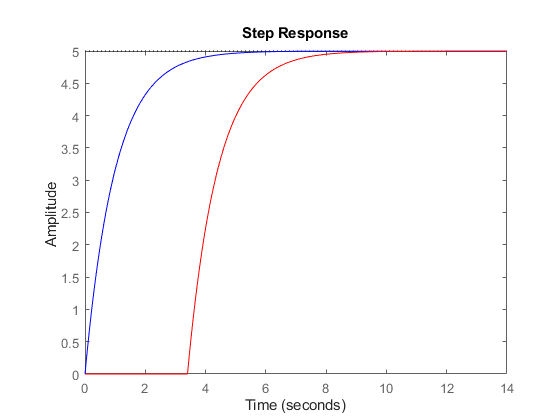
As expected, the step response of P is a shifted version of the delay-free response:
P0 = tf(num,den);
step(P0,'b',P,'r')
If the process model has multiple outputs, for example:
![$$P(s) = \left[\matrix{{5 e^{-3.4 s} \over s+1} \cr {-2 e^{-2.7 s} \over s+3} }\right] , $$](../../examples/control/win64/GSSpecifyingDelays_eq00893717195762289334.png)
you can use the OutputDelay property to specify a different delay for each output channel:
num = {5 ; -2};
den = {[1 1] ; [1 3]};
P = tf(num,den,'OutputDelay',[3.4 ; 2.7])
P =

  From input to output...
                       5
   1:  exp(-3.4*s) * -----
                     s + 1

                      -2
   2:  exp(-2.7*s) * -----
                     s + 3

Continuous-time transfer function.
Next consider a multi-input, multi-output model, e.g.,
![$$P(s) = \left[\matrix{{5 e^{-3.4 s} \over s+1} & 1 \cr {-2 e^{-2.7 s} \over s+3} & {e^{-0.7 s} \over s} }\right] . $$](../../examples/control/win64/GSSpecifyingDelays_eq16391647133053614266.png)
Here the delays are different for each I/O pair, so you must use the IODelay property:
num = {5 , 1; -2 1};
den = {[1 1] , 1; [1 3], [1 0]};
P = tf(num,den,'IODelay',[3.4  0;2.7 0.7]);
A more direct and literal way to specify this model is to introduce the Laplace variable "s" and use transfer function arithmetic:
s = tf('s');
P = [ 5*exp(-3.4*s)/(s+1) , 1 ; -2*exp(-2.7*s)/(s+3) , exp(-0.7*s)/s ]
P =

  From input 1 to output...
                       5
   1:  exp(-3.4*s) * -----
                     s + 1

                      -2
   2:  exp(-2.7*s) * -----
                     s + 3

  From input 2 to output...
   1:  1

                     1
   2:  exp(-0.7*s) * -
                     s

Continuous-time transfer function.
Note that in this case, MATLAB® automatically decides how to distribute the delays between the InputDelay, OutputDelay, and IODelay properties.
P.InputDelay
P.OutputDelay
P.IODelay
ans =

     0
     0


ans =

         0
    0.7000


ans =

    3.4000         0
    2.0000         0
The function totaldelay sums up the input, output, and I/O delay values to give back the values we entered:
totaldelay(P)
ans =

    3.4000         0
    2.7000    0.7000
State-Space Models with Input and Output Delays
Consider the state-space model:

Note that the input signal u(t) is delayed by 2.5 seconds. To specify this model, enter:
sys = ss(-1,1,12,0,'InputDelay',2.5)
sys =

  A =
       x1
   x1  -1

  B =
       u1
   x1   1

  C =
       x1
   y1  12

  D =
       u1
   y1   0

  Input delays (seconds): 2.5

Continuous-time state-space model.
A related model is

Here the 2.5 second delay is at the output, as seen by rewriting these state equations as:

You can therefore specify this model as:
sys1 = ss(-1,1,12,0,'OutputDelay',2.5);
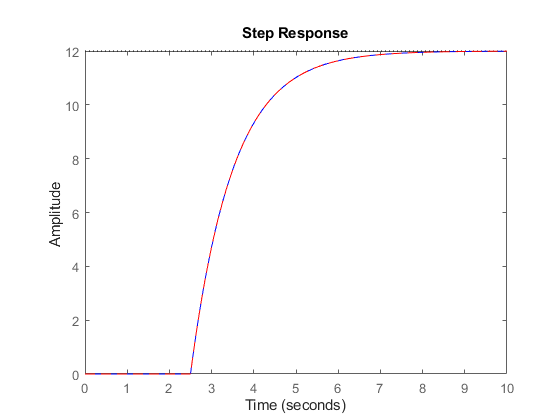
Note that both models have the same I/O response as confirmed by
step(sys,'b',sys1,'r--')
However, their state trajectories are not the same because the states x and x1 are related by

Combining Models with I/O Delays
So far we have only considered LTI models with transport delays between specific I/O pairs. While this is enough to model many processes, this class of models is not general enough to analyze most control systems with delays, including simple feedback loops with delays. For example, consider the parallel connection:

The resulting transfer function

cannot be represented as an ordinary transfer function with a delay at the input or output. To represent  , we must switch to the state-space representation and use the notion of "internal delay". State-space (SS) models have the ability to keep track of delays when connecting systems together. Structural information on the delay location and their coupling with the remaining dynamics is encoded in an efficient and fully general manner. Adding the transfer functions
  and
and  together automatically computes a state-space representation of
  :
:
H1 = 1/(s+2);
H2 = 5*exp(-3.4*s)/(s+1);
H = H1 + H2
H =

  A =
       x1  x2
   x1  -2   0
   x2   0  -1

  B =
       u1
   x1   1
   x2   2

  C =
        x1   x2
   y1    1  2.5

  D =
       u1
   y1   0

  (values computed with all internal delays set to zero)

  Internal delays (seconds): 3.4

Continuous-time state-space model.
Note that
The delay value of 3.4 is listed as "internal"
The A,B,C,D data corresponds to the dynamics when all delays are set to zero (zero-order Pade approximation)
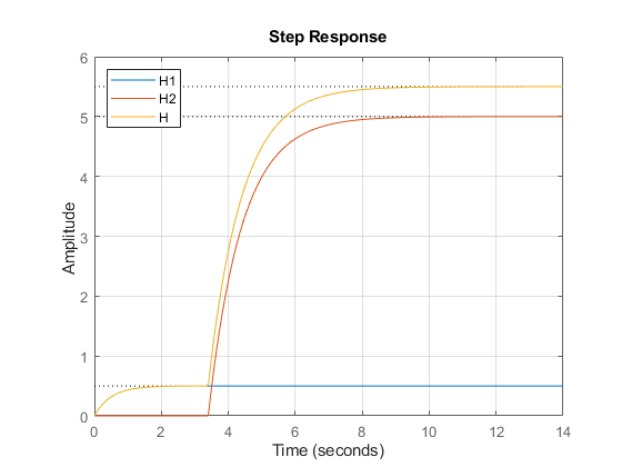
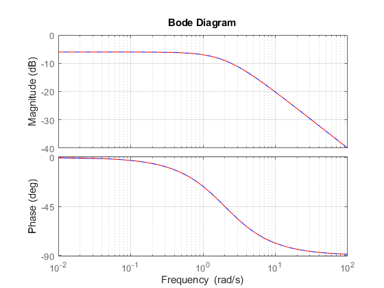
It is neither possible nor advisable to look at the transfer function of models with internal delays. Instead, use time and frequency plots to compare and validate models:
step(H1,H2,H)
legend('H1','H2','H','Location','NorthWest'), grid
bode(H1,'b',H-H2,'r--')  % verify that H-H2 = H1
grid
Building Models with Internal Delays
Typically, state-space models with internal delays are not created by specifying A,B,C,D data together with a set of internal delays. Rather, you build such models by connecting simpler LTI models (some with I/O delays) in series, parallel, or feedback. There is no limitation on how many delays are involved and how the LTI models are connected together.
For example, consider the control loop shown below, where the plant is modeled as a first-order plus dead time.

Figure 1: Feedback Loop with Delay.
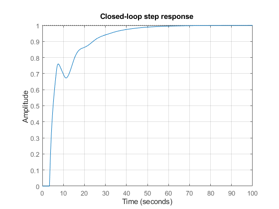
Using the state-space representation, you can derive a model T for the closed-loop response from r to y and simulate it by
P = 5*exp(-3.4*s)/(s+1);
C = 0.1 * (1 + 1/(5*s));
T = feedback(P*C,1);

step(T,100)
grid, title('Closed-loop step response')
For more complicated interconnections, you can name the input and output signals of each block and use connect to automatically take care of the wiring. Suppose, for example, that you want to add feedforward to the control loop of Figure 1:
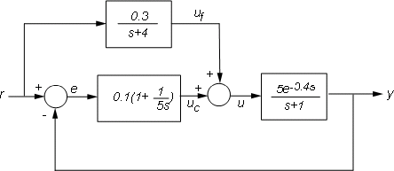
Figure 2: Feedforward and Feedback Control.
You can derive the corresponding closed-loop model T by
F = 0.3/(s+4);
P.u = 'u';  P.y = 'y';
C.u = 'e';  C.y = 'uc';
F.u = 'r';  F.y = 'uf';
Sum1 = sumblk('e = r-y');
Sum2 = sumblk('u = uf+uc');
Tff = connect(P,C,F,Sum1,Sum2,'r','y');
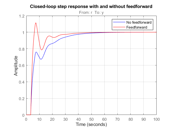
and compare its response with the feedback only design:
step(T,'b',Tff,'r',100)
legend('No feedforward','Feedforward')
grid, title('Closed-loop step response with and without feedforward')
State-Space Equations with Delayed Terms
A special class of LTI models with delays are state-space equations with delayed terms. The general form is


The function delayss helps you specify such models. For example, consider

To create this model, specify Aj,Bj,Cj,Dj for each delay and use delayss to assemble the model:
DelayT(1) = struct('delay',0.5,'a',0,'b',2,'c',1,'d',0);   % tau1=0.5
DelayT(2) = struct('delay',1.2,'a',-1,'b',0,'c',0,'d',0);  % tau2=1.2
sys = delayss(-1,0,0,1,DelayT)
sys =

  A =
       x1
   x1  -2

  B =
       u1
   x1   2

  C =
       x1
   y1   1

  D =
       u1
   y1   1

  (values computed with all internal delays set to zero)

  Internal delays (seconds): 0.5  0.5  1.2

Continuous-time state-space model.
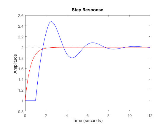
Note that the A,B,C,D values are for all delays set to zero. The response for these values need not be close to the actual response with delays:
step(sys,'b',pade(sys,0),'r')
Discrete-Time Models with Delays
Discrete-time delays are handled in a similar way with some minor differences:
Discrete-time delays are always integer multiples of the sampling period
Discrete-time delays are equivalent to poles at z=0, so it is always possible to absorb delays into the model dynamics. However, keeping delays separate is better for performance, especially for systems with long delays compared to the sampling period.
To specify the first-order model

with sampling period Ts=0.1, use
H = tf(2,[1 -0.95],0.1,'inputdelay',25)
step(H)
H =

               2
  z^(-25) * --------
            z - 0.95

Sample time: 0.1 seconds
Discrete-time transfer function.
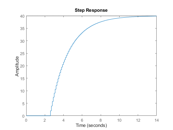
The equivalent state-space representation is
H = ss(H)
H =

  A =
         x1
   x1  0.95

  B =
       u1
   x1   2

  C =
       x1
   y1   1

  D =
       u1
   y1   0

  Input delays (sampling periods): 25

Sample time: 0.1 seconds
Discrete-time state-space model.
Note that the delays are kept separate from the poles. Next, consider the feedback loop below where g is a pure gain.

Figure 3: Discrete-Time Feedback Loop.
To compute the closed-loop response for g=0.01, type
g = .01;
T = feedback(g*H,1)
step(T)
T =

  A =
         x1
   x1  0.93

  B =
       u1
   x1   2

  C =
         x1
   y1  0.01

  D =
       u1
   y1   0

  (values computed with all internal delays set to zero)

  Internal delays (sampling periods): 25

Sample time: 0.1 seconds
Discrete-time state-space model.
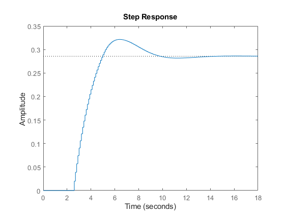
Note that T is still a first-order model with an internal delay of 25 samples. For comparison, map all delays to poles at z=0 using absorbDelay:
T1 = absorbDelay(T);
order(T1)
ans =

    26
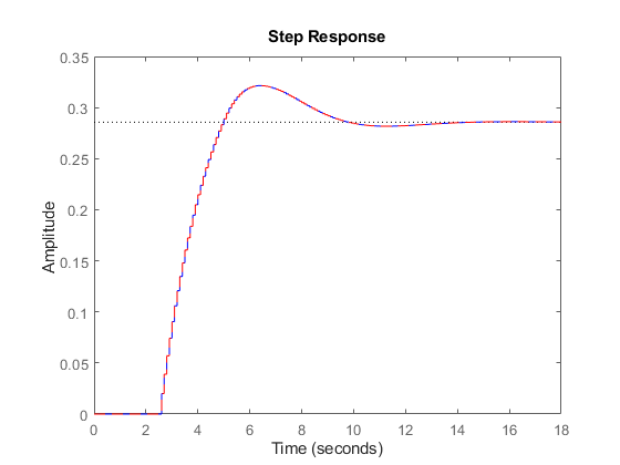
The resulting model has 26 states and is therefore less efficient to simulate. Note that the step responses of T and T1 exactly match as expected:
step(T,'b',T1,'r--')
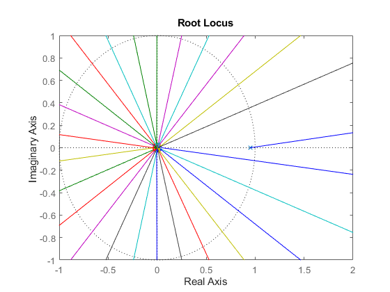
In general, it is recommended to keep delays separate except when analyzing the closed-loop dynamics of models with internal delays:
rlocus(H)
axis([-1 2 -1 1])
Inside State-Space Models with Internal Delays
State-space objects use generalized state-space equations to keep track of internal delays. Conceptually, such models consist of two interconnected parts:
An ordinary state-space model
H(s)with augmented I/O setA bank of internal delays.
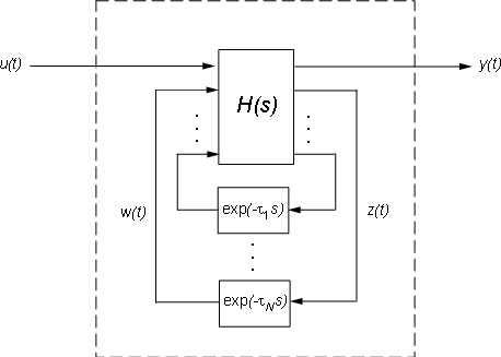
Figure 4: Internal Representation of State-Space Models with Internal Delays.
The corresponding state-space equations are

You need not bother with this internal representation to use the tools. However, if for some reason you want to extract H or the matrices A,B1,B2,..., you can do this with getDelayModel. For the example
P = 5*exp(-3.4*s)/(s+1);
C = 0.1 * (1 + 1/(5*s));
T = feedback(P*C,1);

[H,tau] = getDelayModel(T,'lft');
size(H)
State-space model with 2 outputs, 2 inputs, and 2 states.
Note that H is a two-input, two-output model whereas T is SISO. The inverse operation (combining H and tau to construct T) is performed by setDelayModel.