Tune MIMO Control System for Specified Bandwidth
This example shows how to tune the following control system to achieve a loop crossover frequency between 0.1 and 1 rad/s using looptune.

The plant, G, is a two-input, two-output model (y is a two-element vector signal). For this example, the transfer function of G is given by:
This sample plant is based on the distillation column described in more detail in the example Decoupling Controller for a Distillation Column.
To tune this control system, you first create a numeric model of the plant. Then you create tunable models of the controller elements and interconnect them to build a controller model. Then you use looptune to tune the free parameters of the controller model. Finally, examine the performance of the tuned system to confirm that the tuned controller yields desirable performance.
Create a model of the plant.
s = tf('s');
G = 1/(75*s+1)*[87.8 -86.4; 108.2 -109.6];
G.InputName = {'qL','qV'};
G.OutputName = 'y';
When you tune the control system, looptune uses the channel names G.InputName and G.OutputName to interconnect the plant and controller. Therefore, assign these channel names to match the illustration. When you set G.OutputName = 'y', the G.OutputName is automatically expanded to {'y(1)';'y(2)'}. This expansion occurs because G is a two-output system.
Represent the components of the controller.
D = tunableGain('Decoupler',eye(2));
D.InputName = 'e';
D.OutputName = {'pL','pV'};

PI_L = tunablePID('PI_L','pi');
PI_L.InputName = 'pL';
PI_L.OutputName = 'qL';

PI_V = tunablePID('PI_V','pi');
PI_V.InputName = 'pV';
PI_V.OutputName = 'qV';

sum1 = sumblk('e = r - y',2);
The control system includes several tunable control elements. PI_L and PI_V are tunable PI controllers. These elements represented by tunablePID models. The fixed control structure also includes a decoupling gain matrix D, represented by a tunable tunableGain model. When the control system is tuned, D ensures that each output of G tracks the corresponding reference signal r with minimal crosstalk.
Assigning InputName and OutputName values to these control elements allows you to interconnect them to create a tunable model of the entire controller C as shown.
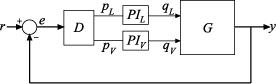
When you tune the control system, looptune uses these channel names to interconnect C and G. The controller C also includes the summing junction sum1. This a two-channel summing junction, because r and y are vector-valued signals of dimension 2.
Connect the controller components.
C0 = connect(PI_L,PI_V,D,sum1,{'r','y'},{'qL','qV'});C0 is a tunable genss model that represents the entire controller structure. C0 stores the tunable controller parameters and contains the initial values of those parameters.
Tune the control system.
The inputs to looptune are G and C0, the plant and initial controller models that you created. The input wc = [0.1,1] sets the target range for the loop bandwidth. This input specifies that the crossover frequency of each loop in the tuned system fall between 0.1 and 1 rad/min.
wc = [0.1,1];
[G,C,gam,Info] = looptune(G,C0,wc);
Final: Peak gain = 0.981, Iterations = 26
Achieved target gain value TargetGain=1.
The displayed Peak Gain = 0.949 indicates that looptune has found parameter values that achieve the target loop bandwidth. looptune displays the final peak gain value of the optimization run, which is also the output gam. If gam is less than 1, all tuning requirements are satisfied. A value greater than 1 indicates failure to meet some requirement. If gam exceeds 1, you can increase the target bandwidth range or relax another tuning requirement.
looptune also returns the tuned controller model C. This model is the tuned version of C0. It contains the PI coefficients and the decoupling matrix gain values that yield the optimized peak gain value.
Display the tuned controller parameters.
showTunable(C)
Decoupler =

  D =
            u1       u2
   y1    1.231  -0.8807
   y2   -1.515    1.237

Name: Decoupler
Static gain.
-----------------------------------
PI_L =

             1
  Kp + Ki * ---
             s

  with Kp = 2.25, Ki = 0.127

Name: PI_L
Continuous-time PI controller in parallel form.
-----------------------------------
PI_V =

             1
  Kp + Ki * ---
             s

  with Kp = -1.79, Ki = -0.0885

Name: PI_V
Continuous-time PI controller in parallel form.
Check the time-domain response for the control system with the tuned coefficients. To produce a plot, construct a closed-loop model of the tuned control system. Plot the step response from reference to output.
T = connect(G,C,'r','y');
step(T)
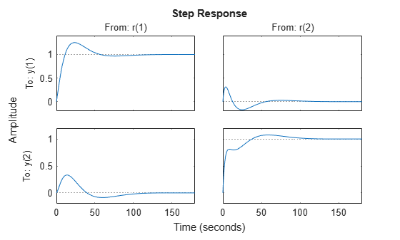
The decoupling matrix in the controller permits each channel of the two-channel output signal y to track the corresponding channel of the reference signal r, with minimal crosstalk. From the plot, you can see how well this requirement is achieved when you tune the control system for bandwidth alone. If the crosstalk still exceeds your design requirements, you can use a TuningGoal.Gain requirement object to impose further restrictions on tuning.
Examine the frequency-domain response of the tuned result as an alternative method for validating the tuned controller.
figure('Position',[100,100,520,1000])
loopview(G,C,Info)
The first plot shows that the open-loop gain crossovers fall within the specified interval [0.1,1]. This plot also includes the maximum and tuned values of the sensitivity function and complementary sensitivity . The second and third plots show that the MIMO stability margins of the tuned system (blue curve) do not exceed the upper limit (yellow curve).