Chebyshev Spline Construction
This section discusses these aspects of the Chebyshev spline construction:
What Is a Chebyshev Spline?
The Chebyshev spline C=Ct=Ck,t of order k for the knot sequence t=(ti: i=1:n+k) is the unique element of Sk,t of max-norm 1 that maximally oscillates on the interval [tk..tn+1] and is positive near tn+1. This means that there is a unique strictly increasing n-sequence τ so that the function C=Ct∊Sk,t given by C(τi)=(–1)n – 1, all i, has max-norm 1 on [tk..tn+1]. This implies that τ1=tk,τn=tn+1, and that ti < τi < tk+i, for all i. In fact, ti+1 ≤ τi ≤ ti+k–1, all i. This brings up the point that the knot sequence is assumed to make such an inequality possible, i.e., the elements of Sk,t are assumed to be continuous.
In short, the Chebyshev spline C looks just like
the Chebyshev
polynomial. It performs similar functions. For example, its extreme
sites τ are particularly good
sites to interpolate at from Sk,t because
the norm of the resulting projector is about as small as can be; see
the toolbox command chbpnt.
You can run the example Construct Chebyshev Spline to construct C for a particular knot sequence t.
Choice of Spline Space
You deal with cubic splines, i.e., with order
k = 4;
and use the break sequence
breaks = [0 1 1.1 3 5 5.5 7 7.1 7.2 8];
lp1 = length(breaks);
and use simple interior knots, i.e., use the knot sequence
t = breaks([ones(1,k) 2:(lp1-1) lp1(:,ones(1,k))]);
n = length(t)-k;
Note the quadruple knot at each end. Because k = 4,
this makes [0..8] = [breaks(1)..breaks(lp1)]
the interval [tk..tn+1]
of interest, with n = length(t)-k the
dimension of the resulting spline space Sk,t.
The same knot sequence would have been supplied by
t=augknt(breaks,k);
Initial Guess
As the initial guess for the τ, use the knot averages
recommended as good interpolation site choices. These are supplied by
tau=aveknt(t,k);
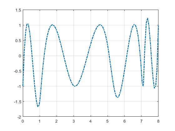
Plot the resulting first approximation to C, i.e., the spline c that satisfies c(τi)=(–1)n-–i, all i:
b = cumprod(repmat(-1,1,n)); b = b*b(end);
c = spapi(t,tau,b);
fnplt(c,'-.')
grid
Here is the resulting plot.
First Approximation to a Chebyshev Spline
Remez Iteration
Starting from this approximation, you use the Remez algorithm to produce a sequence of splines converging to C. This means that you construct new τ as the extrema of your current approximation c to C and try again. Here is the entire loop.
Find the new interior τi as the zeros of Dc—that is, the first derivative of c. First, differentiate
Dc = fnder(c);
Take the zeros of Dc using the fnzeros function. The
zeros represent the extrema of the current approximation c. The result is
the new guess for tau.
tau(2:n-1) = mean(fnzeros(Dc));
Then check the extrema values of your current approximation there:
extremes = abs(fnval(c, tau));
The difference
max(extremes)-min(extremes)
  ans = 0.6906
is an estimate of how far you are from total leveling.
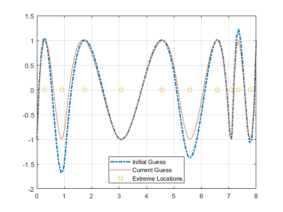
Construct a new spline corresponding to the new choice of tau and
plot it on top of the old:
c = spapi(t,tau,b);
sites = sort([tau (0:100)*(t(n+1)-t(k))/100]);
values = fnval(c,sites);
hold on, plot(sites,values)
The following code turns on the grid and plots the locations of the extrema.
grid on
plot(tau(2:end-1),zeros(size(tau(2:end-1))),'o');
hold off
lgd = legend( 'Initial Guess', 'Current Guess', 'Extreme Locations',...
 'location', 'NorthEastOutside' );
lgd.Location = 'south';
Following is the resulting figure (legend not shown).
A More Nearly Level Spline
If this is not close enough, one simply reiterates the loop. For this example, the next iteration already produces C to graphic accuracy.