fntlr
Taylor coefficients
Syntax
taylor = fntlr(f,dorder,x)
Description
taylor = fntlr(f,dorder,x) returns the nonnormalized Taylor coefficients, up to the given order dorder and at the given x, of the function described in f.
For a univariate function and a scalar x, this is the vector
If, more generally, the function in f is d-valued with d>1 or even prod(d)>1 and/or is m-variate for some m>1, then dorder is expected to be an m-vector of positive integers, x is expected to be a matrix with m rows, and, in that case, the output is of size [prod(d)*prod(dorder),size(x,2)], with its j-th column containing
for i1=1:dorder(1), ..., im=1:dorder(m). Here, Dif is the partial derivative of f with respect to its ith argument.
Examples
If f contains a univariate function and x is a scalar or a 1-row matrix, then fntlr(f,3,x) produces the same output as the statements
df = fnder(f); [fnval(f,x); fnval(df,x); fnval(fnder(df),x)];
As a more complicated example, look at the Taylor vectors of order 3 at 21 equally spaced points for the rational spline whose graph is the unit circle:
ci = rsmak('circle'); in = fnbrk(ci,'interv');
t = linspace(in(1),in(2),21); t(end)=[];
v = fntlr(ci,3,t);
We plot ci along with the points v(1:2,:), to verify that these are, indeed, points on the unit circle.
fnplt(ci), hold on, plot(v(1,:),v(2,:),'o')
Next, to verify that v(3:4,j) is a vector tangent to the circle at the point v(1:2,j), we use the MATLAB® quiver command to add the corresponding arrows to our plot:
quiver(v(1,:),v(2,:),v(3,:),v(4,:))
Finally, what about v(5:6,:)? These are second derivatives, and we add the corresponding arrows by the following quiver command, thus finishing First and Second Derivative of a Rational Spline Giving a Circle.
quiver(v(1,:),v(2,:),v(5,:),v(6,:)), axis equal, hold off
First and Second Derivative of a Rational Spline Giving a Circle
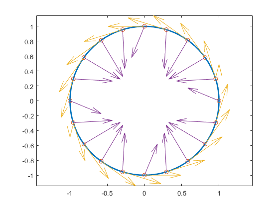
Now, our curve being a circle, you might have expected the 2nd derivative arrows to point straight to the center of that circle, and that would have been indeed the case if the function in ci had been using arclength as its independent variable. Since the parameter used is not arclength, we use the formula, given in Example: B-form Spline Approximation to a Circle, to compute the curvature of the curve given by ci at these selected points. For ease of comparison, we switch over to the variables used there and then simply use the commands from there.
dspt = v(3:4,:); ddspt = v(5:6,:);
kappa = abs(dspt(1,:).*ddspt(2,:)-dspt(2,:).*ddspt(1,:))./...
   (sum(dspt.^2)).^(3/2);
max(abs(kappa-1))
ans = 2.2204e-016
The numerical answer is reassuring: at all the points tested, the curvature is 1 to within roundoff.