rscvn
Piecewise biarc Hermite interpolation
Syntax
c = rscvn(p,u)

c = rscvn(p)
Description
c = rscvn(p,u) returns a planar piecewise biarc curve (in quadratic rBform) that passes, in order, through the given points p(:,j) and is constructed in the following way (see Construction of a Biarc). Between any two distinct points p(:,j) and p(:,j+1), the curve usually consists of two circular arcs (including straight-line segments) which join with tangent continuity, with the first arc starting at p(:,j) and normal there to u(:,j), and the second arc ending at p(:,j+1) and normal there to u(:,j+1), and with the two arcs written as one whenever that is possible. Thus the curve is tangent-continuous everywhere except, perhaps, at repeated points, where the curve may have a corner, or when the angle, formed by the two segments ending at p(:,j), is unusually small, in which case the curve may have a cusp at that point.
p must be a real matrix, with two rows, and at least two columns, and any column must be different from at least one of its neighboring columns.
u must be a real matrix with two rows, with the same number of columns as p (for two exceptions, see below), and can have no zero column.
c = rscvn(p) chooses the normals in the following way. For j=2:end-1, u(:,j) is the average of the (normalized, right-turning) normals to the vectors p(:,j)-p(:,j-1) and p(:,j+1)-p(:,j). If p(:,1)==p(:,end), then both end normals are chosen as the average of the normals to p(:,2)-p(:,1) and p(:,end)-p(:,end-1) thus preventing a corner in the resulting closed curve. Otherwise, the end normals are so chosen that there is only one arc over the first and last segment (not-a-knot end condition).
rscvn(p,u), with u having exactly two columns, also chooses the interior normals as for the case when u is absent but uses the two columns of u as the end-point normals.
Examples
Example 1. The following code generates a description of a circle, using just four pieces. Except for a different scaling of the knot sequence, it is the same description as is supplied by rsmak('circle',1,[1;1]).
p = [1 0 -1 0 1; 0 1 0 -1 0]; c = rscvn([p(1,:)+1;p(2,:)+1],p);
The same circle, but using just two pieces, is provided by
c2 = rscvn([0,2,0; 1,1,1]);
Example 2. The following code plots two letters. Note that the second letter is the result of interpolation to just four points. Note also the use of translation in the plotting of the second letter.
p = [-1 .8 -1 1 -1 -1 -1; 3 1.75 .5 -1.25 -3 -3  3];
i = eye(2); u = i(:,[2 1 2 1 2 1 1]); B = rscvn(p,u);
S = rscvn([1 -1 1 -1; 2.5 2.5 -2.5 -2.5]);
fnplt(B), hold on, fnplt(fncmb(S,[3;0])), hold off
axis equal, axis off
Two Letters Composed of Circular Arcs
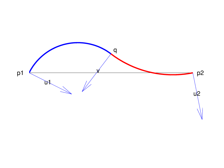
Example 3. The following code generates the Construction of a Biarc, of use in the discussion below of the biarc construction used here. Note the use of fntlr to find the tangent to the biarc at the beginning, at the point where the two arcs join, and at the end.
p = [0 1;0 0];  u = [.5 -.1;-.25 .5];
plot(p(1,:),p(2,:),'k'), hold on
biarc = rscvn(p,u); breaks = fnbrk(biarc,'b');
fnplt(biarc,breaks(1:2),'b',3), fnplt(biarc,breaks(2:3),'r',3)
vd = fntlr(biarc,2,breaks);
quiver(vd(1,:),vd(2,:),vd(4,:),-vd(3,:)), hold off
Construction of a Biarc
Algorithms
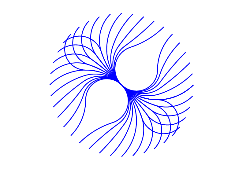
Given two distinct points, p1 and p2, in the plane and, correspondingly, two nonzero vectors, u1 and u2, there is a one-parameter family of biarcs (i.e., a curve consisting of two arcs with common tangent at their join) starting at p1 and normal there to u1 and ending at p2 and normal there to u2. One way to parametrize this family of biarcs is by the normal direction, v, at the point q at which the two arcs join. With a nonzero v chosen, there is then exactly one choice of q, hence the entire biarc is then determined. In the construction used in rscvn, v is chosen as the reflection, across the perpendicular to the segment from p1 to p2, of the average of the vectors u1 and u2, -- after both vectors have been so normalized that their length is 1 and that they both point to the right of the segment from p1 to p2. This choice for v seems natural in the two standard cases: (i) u2 is the reflection of u1 across the perpendicular to the segment from p1 to p2; (ii) u1 and u2 are parallel. This choice of v is validated by Biarcs as a Function of the Left Normal which shows the resulting biarcs when p1, p2, and u2 = [.809;.588]are kept fixed and only the normal at p1 is allowed to vary.
Biarcs as a Function of the Left Normal
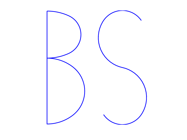
But it is impossible to have the interpolating biarc depend continuously at all four data, p1, p2, u1, u2. There has to be a discontinuity as the normal directions, u1 and u2, pass through the direction from p1 to p2. This is illustrated in Biarcs as a Function of One Endpoint which shows the biarcs when one point, p1 = [0;0], and the two normals, u1 = [1;1] and u2 = [1;-1], are held fixed and only the other point, p2, moves, on a circle around p1.
Biarcs as a Function of One Endpoint