Run Sequence-to-Sequence Regression on FPGAs
This example shows how to create, compile, and deploy a long short-term memory (LSTM) network trained on remaining useful life (RUL) of engines. Use the deployed network to predict the RUL for an engine. Use MATLAB® to retrieve the prediction results from the target device.
This example uses the turbofan engine degradation data used in [1]. The example uses an LSTM network to predict the remaining useful life of an engine measured in cycles when given time series data representing various sensors in the engine. The training data contains simulated time series data for 100 engines. Each sequence varies in length and corresponds to a full run to failure (RTF) instance. The test data contains 100 partial sequences and the corresponding values for the remaining useful life at the end of each sequence.
The data set contains 100 training observations and 100 test observations.
To learn more about how to train this network, see Sequence-to-Sequence Regression Using Deep Learning. For this example, you must have a Xilinx® Zynq® Ultrascale+™ ZCU102 SoC development kit.
Download Data
Download and unzip the turbofan engine degradation simulation data set.
Each time series in the turbofan engine degradation simulation data set represents a different engine. Each engine starts with unknown degrees of initial wear and manufacturing variation. The engine operates normally at the start of each time series, and develops a fault at some point during the series. In the training set, the fault grows in magnitude until system failure.
The data contains ZIP-compressed text files with 26 columns of numbers, separated by spaces. Each row is a snapshot of data taken during a single operational cycle, and each column is a different variable. The columns correspond to the following:
Column 1 — Unit number
Column 2 — Time in cycles
Columns 3–5 — Operational settings
Columns 6–26 — Sensor measurements 1–21
Create a directory to store the turbofan engine degradation Simulation data set.
dataFolder = fullfile(tempdir,"turbofan");
if ~exist(dataFolder,'dir')
    mkdir(dataFolder);
end
Download and extract the turbofan engine degradation simulation data set.
filename = matlab.internal.examples.downloadSupportFile("nnet","data/TurbofanEngineDegradationSimulationData.zip");
unzip(filename,dataFolder)
Prepare Test Data
Load the test data using the processTurboFanDataTest function attached to this example. The processTurboFanDataTest function extracts the data from filenamePredictors and filenameResponses and returns the cell arrays XTest and YTest, which contain the test predictor and response sequences, respectively.
filenamePredictors = fullfile(pwd,"test_FD001.txt");
filenameResponses = fullfile(pwd,"RUL_FD001.txt");
[XTest,YTest] = processTurboFanDataTest(filenamePredictors,filenameResponses);
Remove features with constant values using idxConstant calculated from the training data. Normalize the test predictors using the same parameters as in the training data. Clip the test responses at the same threshold used for the training data.
filenamePredictors = fullfile(pwd,"train_FD001.txt");
[XTrain,YTrain] = processTurboFanDataTrain(filenamePredictors);
Remove Features with Constant Values
Features that remain constant for all time steps can negatively impact the training. Find the rows of data that have the same minimum and maximum values, and remove the rows. Then use these values to clean up the test dataset.
m = min([XTrain{:}],[],2);
M = max([XTrain{:}],[],2);
idxConstant = M == m;

for i = 1:numel(XTrain)
    XTrain{i}(idxConstant,:) = [];
end

numFeatures = size(XTrain{1},1);
mu = mean([XTrain{:}],2);
sig = std([XTrain{:}],0,2);

for i = 1:numel(XTrain)
    XTrain{i} = (XTrain{i} - mu) ./ sig;
end

thr = 150; %threshold
for i = 1:numel(XTest)
    XTest{i}(idxConstant,:) = [];
    XTest{i} = (XTest{i} - mu) ./ sig;
    YTest{i}(YTest{i} > thr) = thr;
end
Load the Pretrained Network
Load the LSTM network. This network was trained on NASA CMAPSS Data described in [1], enter:
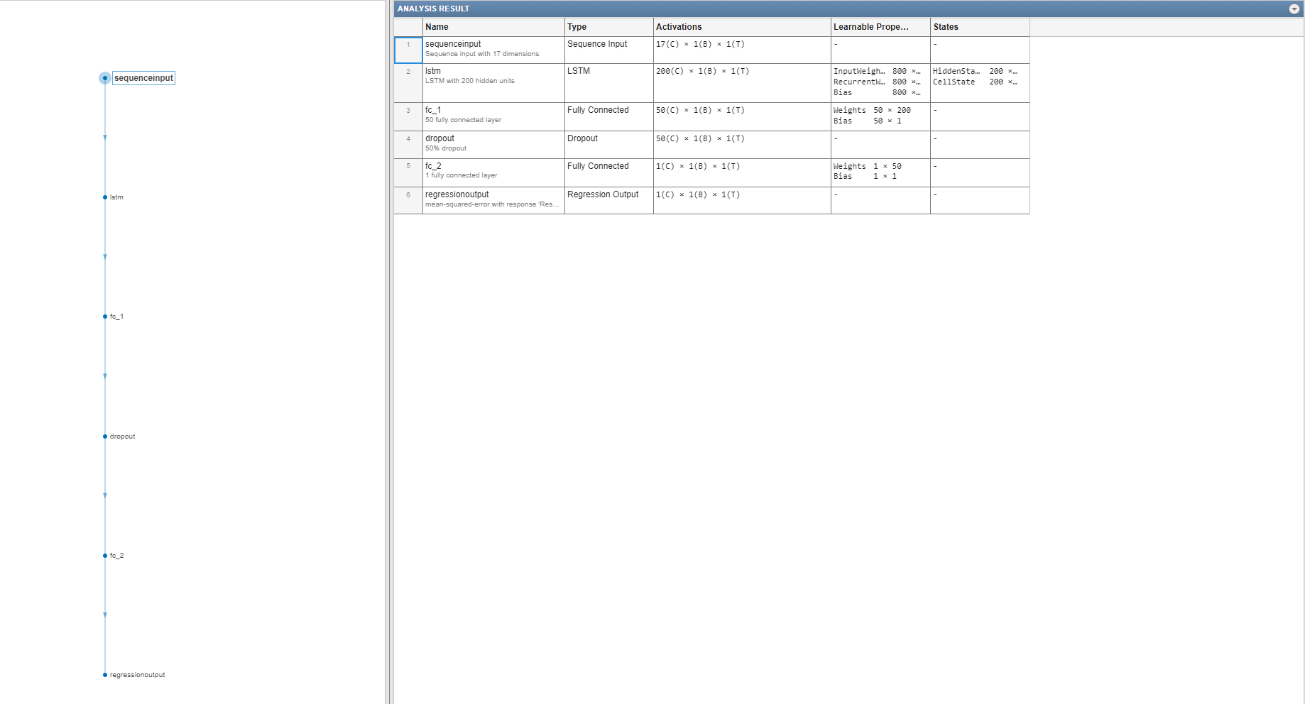
load CMAPSSDataNetworkView the layers of the network by using the analyzeNetwork function. The function returns a graphical representation of the network and the parameter settings for the layers in the network.
analyzeNetwork(net)
Define FPGA Board Interface
Define the target FPGA board programming interface by using the dlhdl.Target object. Specify that the interface is for a Xilinx board with an Ethernet interface.
To create the target object, enter:
hTarget = dlhdl.Target('Xilinx','Interface','Ethernet');
Alternatively, to use the JTAG interface, install Xilinx™ Vivado™ Design Suite 2020.2. To set the Xilinx Vivado toolpath, enter:
hdlsetuptoolpath('ToolName', 'Xilinx Vivado', 'ToolPath', 'C:\Xilinx\Vivado\2020.2\bin\vivado.bat');
hTarget = dlhdl.Target('Xilinx','Interface','JTAG');
Prepare Network for Deployment
Prepare the network for deployment by creating a dlhdl.Workflow object. Specify the network and the bitstream name. Ensure that the bitstream name matches the data type of your FPGA board. In this example, the target board is the Xilinx ZCU102 SOC. The bitstream uses a single data type.
hW = dlhdl.Workflow('network', net, 'Bitstream', 'zcu102_lstm_single','Target',hTarget);
Alternatively, to run the example on the Xilinx ZC706 board, enter:
hW = dlhdl.Workflow('Network', snet, 'Bitstream', 'zc706_lstm_single','Target',hTarget);
Compile Network
Run the compile method of the dlhdl.Workflow object to compile the network and generate the instructions, weights, and biases for deployment. The total number of frames exceeds the default value of 30. Set the InputFrameNumberLimit name-value argument to 500 to run predictions in chunks of 500 frames to prevent timeouts.
dn = compile(hW,'InputFrameNumberLimit',500)### Compiling network for Deep Learning FPGA prototyping ...
### Targeting FPGA bitstream zcu102_lstm_single.
### The network includes the following layers:
1 'sequenceinput' Sequence Input Sequence input with 17 dimensions (SW Layer)
2 'lstm' LSTM LSTM with 200 hidden units (HW Layer)
3 'fc_1' Fully Connected 50 fully connected layer (HW Layer)
4 'fc_2' Fully Connected 1 fully connected layer (HW Layer)
5 'regressionoutput' Regression Output mean-squared-error with response 'Response' (SW Layer)
### Notice: The layer 'sequenceinput' with type 'nnet.cnn.layer.ImageInputLayer' is implemented in software.
### Notice: The layer 'regressionoutput' with type 'nnet.cnn.layer.RegressionOutputLayer' is implemented in software.
### Compiling layer group: lstm.wi ...
### Compiling layer group: lstm.wi ... complete.
### Compiling layer group: lstm.wo ...
### Compiling layer group: lstm.wo ... complete.
### Compiling layer group: lstm.wg ...
### Compiling layer group: lstm.wg ... complete.
### Compiling layer group: lstm.wf ...
### Compiling layer group: lstm.wf ... complete.
### Compiling layer group: fc_1>>fc_2 ...
### Compiling layer group: fc_1>>fc_2 ... complete.
### Allocating external memory buffers:
offset_name offset_address allocated_space
_______________________ ______________ __________________
"InputDataOffset" "0x00000000" "40.0 kB"
"OutputResultOffset" "0x0000a000" "8.0 kB"
"SchedulerDataOffset" "0x0000c000" "596.0 kB"
"SystemBufferOffset" "0x000a1000" "20.0 kB"
"InstructionDataOffset" "0x000a6000" "4.0 kB"
"FCWeightDataOffset" "0x000a7000" "736.0 kB"
"EndOffset" "0x0015f000" "Total: 1404.0 kB"
### Network compilation complete.
dn = struct with fields:
             weights: [1×1 struct]
        instructions: [1×1 struct]
           registers: [1×1 struct]
    syncInstructions: [1×1 struct]
        constantData: {}
             ddrInfo: [1×1 struct]
       resourceTable: [6×2 table]
Program Bitstream onto FPGA and Download Network Weights
To deploy the network on the Xilinx ZCU102 SoC hardware, run the deploy function of the dlhdl.Workflow object. This function uses the output of the compile function to program the FPGA board by using the programming file. The deploy function starts programming the FPGA device and displays progress messages, and the required time to deploy the network.
hW.deploy
### Programming FPGA Bitstream using Ethernet...
### Attempting to connect to the hardware board at 192.168.1.101...
### Connection successful
### Programming FPGA device on Xilinx SoC hardware board at 192.168.1.101...
### Copying FPGA programming files to SD card...
### Setting FPGA bitstream and devicetree for boot...
# Copying Bitstream zcu102_lstm_single.bit to /mnt/hdlcoder_rd
# Set Bitstream to hdlcoder_rd/zcu102_lstm_single.bit
# Copying Devicetree devicetree_dlhdl.dtb to /mnt/hdlcoder_rd
# Set Devicetree to hdlcoder_rd/devicetree_dlhdl.dtb
# Set up boot for Reference Design: 'AXI-Stream DDR Memory Access : 3-AXIM'
### Rebooting Xilinx SoC at 192.168.1.101...
### Reboot may take several seconds...
### Attempting to connect to the hardware board at 192.168.1.101...
### Connection successful
### Programming the FPGA bitstream has been completed successfully.
### Resetting network state.
### Loading weights to FC Processor.
### FC Weights loaded. Current time is 10-Dec-2023 16:56:53
Predict Remaining Useful Life
Run the predict method of the dlhdl.Workflow object, to make predictions on the test data.
YTestPred = predict(hW,XTest{i},Profile='on');### Resetting network state.
### Finished writing input activations.
### Running a sequence of length 198.
Deep Learning Processor Profiler Performance Results
LastFrameLatency(cycles) LastFrameLatency(seconds) FramesNum Total Latency Frames/s
------------- ------------- --------- --------- ---------
Network 87171 0.00040 198 17327757 2513.9
memSeparator_0 99 0.00000
memSeparator_3 237 0.00000
lstm.wi 19328 0.00009
lstm.wo 19287 0.00009
lstm.wg 19288 0.00009
lstm.wf 20325 0.00009
lstm.sigmoid_1 275 0.00000
lstm.sigmoid_3 267 0.00000
lstm.tanh_1 297 0.00000
lstm.sigmoid_2 267 0.00000
lstm.multiplication_2 447 0.00000
lstm.multiplication_1 477 0.00000
lstm.c_add 421 0.00000
lstm.tanh_2 281 0.00000
memSeparator_2 217 0.00000
lstm.multiplication_3 427 0.00000
memSeparator_1 281 0.00000
fc_1 4666 0.00002
fc_2 283 0.00000
* The clock frequency of the DL processor is: 220MHz
 for i = 1:numel(XTest)
 YPred{i} = hW.predict(XTest{i});
end
The LSTM network makes predictions on the partial sequence one time step at a time. At each time step, the network makes predictions using the value at this time step, and the network state calculated from the previous time steps. The network updates its state between each prediction. The predict function returns a sequence of these predictions. The last element of the prediction corresponds to the predicted RUL for the partial sequence.
Alternatively, you can make predictions one time step at a time by using predict and setting the KeepState name-value argument to true. This function is useful when you have the values of the time steps in a stream. Usually, it is faster to make predictions on full sequences when compared to making predictions one time step at a time. For an example showing how to forecast future time steps by updating the network between single time step predictions, see Time Series Forecasting Using Deep Learning.
Visualize some of the predictions in a plot.
idx = randperm(numel(YPred),4);
figure
for i = 1:numel(idx)
    subplot(2,2,i)

    plot(YTest{idx(i)},'--')
    hold on
    plot(YPred{idx(i)},'.-')
    hold off

    ylim([0 thr + 25])
    title("Test Observation " + idx(i))
    xlabel("Time Step")
    ylabel("RUL")
end
legend(["Test Data" "Predicted"],'Location','southeast')

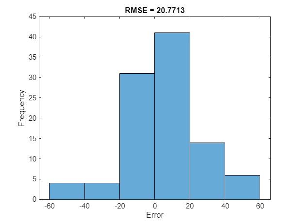
For a given partial sequence, the predicted current RUL is the last element of the predicted sequences. Calculate the root-mean-square error (RMSE) of the predictions and visualize the prediction error in a histogram.
for i = 1:numel(YTest)
    YTestLast(i) = YTest{i}(end);
    YPredLast(i) = YPred{i}(end);
end
figure
rmse = sqrt(mean((YPredLast - YTestLast).^2))
rmse = single

20.7713
histogram(YPredLast - YTestLast)
title("RMSE = " + rmse)
ylabel("Frequency")
xlabel("Error")
References
Saxena, Abhinav, Kai Goebel, Don Simon, and Neil Eklund. "Damage propagation modeling for aircraft engine run-to-failure simulation." 2008 International Conference on Prognostics and Health Management (2008): 1–9. https://doi.org/10.1109/PHM.2008.4711414.
See Also
dlhdl.Target | dlhdl.Workflow | compile | deploy | predict | classify