Custom Training Loops and Loss Functions for AI-Based Wireless Systems

This example shows how to use a custom training loop and a custom loss function for model-free training of an end-to-end communications system as an autoencoder. The autoencoder maps bits to channel optimized symbols and computes log-likelihood ratios (LLRs) for the received bits.

Introduction

The Autoencoders for Wireless Communications (Communications Toolbox) example introduces the basic idea of designing an end-to-end communications system as an autoencoder. The autoencoder assumes that the channel is known and differentiable. In this example, you implement a model-free autoencoder training algorithm for unknown or nondifferentiable channels as shown in [1].

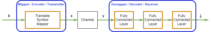
Autoencoders consist of a transmitter and a receiver. The transmitter, also known as the encoder or mapper, maps bits into complex symbols. The receiver, also known as the decoder or demapper, demaps the received complex symbols by estimating LLR values for the transmitted bits. This figure shows an autoencoder with a channel between the encoder and decoder. Assume that an outer code provides the coded bits, $$b$$, and the output of the decoder is the LLR estimates, $$\underset{}{\overset{ˆ}{b}}$$, which the receiver uses to decode the outer code.

During training, you must first pass bits through the encoder, channel, and decoder to obtain the network output. The algorithm then calculates a loss value by comparing the actual output and the expected output. Finally, the algorithm calculates the gradient of the loss function by using the chain rule during backpropagation. The Conventional End-to-End Training of Communications System example shows the design and training of an autoencoder with differentiable channel. If any of the layers, such as the channel layer, is not differentiable, the backpropagation algorithm cannot calculate the gradients for that layer and any layer before that. The model-free training algorithm solves this problem by training the transmitter and receiver separately [1].

This figure shows the model-free training algorithm. The algorithm first trains the receiver in a loop using the loss calculated at the output of the receiver. Then the algorithm adds a known perturbation to the transmitter output and calculates the transmitter loss based on the receiver loss. The algorithm updates the transmitter weights using the transmitter loss together with estimated gradients. Then the algorithm iterates many times until it achieves a satisfactory loss value. Finally, the algorithm fine-tunes the receiver while keeping the transmitter weights the same. In the following sections, you implement this model-free training algorithm by using custom training loops and custom loss functions.

System Parameters

Design a wireless autoencoder that takes $$n$$ bits and outputs $$n/N_{bps}$$ complex symbols, where $$n$$ is codeword length, and $$N_{bps}$$ is the number of bits per symbol. $$n$$ must be an integer multiple of $$N_{bps}$$. Assume an outer code, such an LDPC code, with a code rate of $$1/2$$. Select codeword length as 648 or 1296. Set the number of blocks per frame, $$N_{blk}$$, to 1. A block of bits is a codeword.

bitsPerSymbol  = 6;  % Number of bits per QAM symbol
M              = 2^bitsPerSymbol;
codewordLength = 1296;  % Codeword length (LDPC)
codeRate       = 1/2;                   % Outer code rate (LDPC)
Nblk           = 1;  % Number of blocks (codewords)

Training Parameters

Set batch size, $$N_b$$, to 128. Randomly select $$E_b/N_o$$ values between 5 and 8 dB. Set the initial learning rate to 1e-3. Drop the learning rate by a factor of 0.9 every 2000 training iterations. For other values of $$N_{bps}$$, the scale the $$E_b/N_o$$ values to keep the training symbol error rate (SER) around 10% and adjust initial learning rate. For an $$N_{bps}$$ value of 4, set initial learning rate to 5e-3, ebnoMin to 3.5 and ebnoMax to 6.5.

Nb = 128;
ebnoMin = 5;
ebnoMax = 8;
learningRate = 1e-3;
learningRateDropPeriod = 2000;
learningRateDropFactor = 0.9;

Convert $$E_b/N_o$$ values to $$SNR$$ values.

snrMin = convertSNR(ebnoMin,"ebno", ...
      BitsPerSymbol=bitsPerSymbol, ...
      CodingRate=codeRate);
snrMax = convertSNR(ebnoMax,"ebno", ...
      BitsPerSymbol=bitsPerSymbol, ...
      CodingRate=codeRate);

Transmitter Neural Network

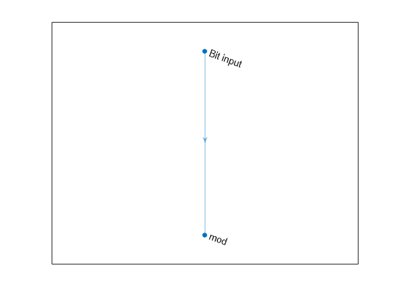
The transmitter network takes a bit sequence as an input and maps the bits to complex symbols using the helperTrainableSymbolMapperLayer function. The helperTrainableSymbolMapperLayer function defines constellation points as a learnable property. Set the modulation order to $$2^{N_{bps}}$$. To prevent the layer from increasing the output power without a bound as a means to reduce symbol errors and loss, set UnitAveragePower to true to enforce unit average power for the constellation. The input to the transmitter is a $$[1\times N_b\times n{N}_{blk}]$$ array. The output of the transmitter is a $$[2\times N_b\times n{N}_{blk}/N_{bps}]$$ array, where the first dimension represents complex symbol values with separate the real and imaginary parts. First value is the real part (in-phase) and the second value is the corresponding imaginary part (quadrature).

layers = [
  sequenceInputLayer(1,Name="Bit input",MinLength=codewordLength*Nblk)
  
  helperTrainableSymbolMapperLayer(ModulationOrder=2^bitsPerSymbol, ...
    BitInput=true, ...
    UnitAveragePower=true, ...
    Name="mod")
  ];
txNet = dlnetwork(layers);
figure
plot(txNet)

Receiver Neural Network

The receiver is a fully connected neural network with two hidden layers and an output layer. The input to the receiver is the channel impaired complex symbols in the form of a $$[1\times N_b\times n{N}_{blk}/N_{bps}]$$ array and $$lo{g}_{10}\left(n_o\right)$$, which is the per batch channel noise variance array in log domain with size $$[1\times N_b]$$. Each hidden layer has 128 outputs followed by ReLU activation. The output layer estimates the LLR values for bits in every symbol in the form of a $$[N_{bps}\times N_b\times n{N}_{blk}]$$ array.

lgraph = layerGraph([
  sequenceInputLayer(1,Name="rcvd symbols",SplitComplexInputs=true, ...
                     MinLength=codewordLength*Nblk/bitsPerSymbol)

  concatenationLayer(1,2,Name="demapper_concat")

  fullyConnectedLayer(128,Name="demapper_fc1")
  reluLayer(Name="demapper_relu1")

  fullyConnectedLayer(128,Name="demapper_fc2")
  reluLayer(Name="demapper_relu2")

  fullyConnectedLayer(bitsPerSymbol,Name="demapper_fc3")
  ]);
noInput = sequenceInputLayer(1,Name="no", ...
                             MinLength=codewordLength*Nblk/bitsPerSymbol);
lgraph = addLayers(lgraph,noInput);
lgraph = connectLayers(lgraph,"no","demapper_concat/in2");
rxNet = dlnetwork(lgraph);
figure
plot(rxNet)

Model-Free Training of Autoencoder

The model-free training algorithm first updates the receiver weights, iterating over the algorithm defined in the Receiver Training section 10 times. Then, the algorithm updates the transmitter weights using the RL-based algorithm described in the Transmitter Training section. The Custom Training Loop section shows the overall training loop that iterates over receiver and transmitter updates.

Receiver Training

This figure shows the conventional training process for optimizing the receiver. Pass the binary data, $$b$$, through the transmitter, channel, and receiver to obtain LLR estimates, $$\underset{}{\overset{ˆ}{b}}$$. Then calculate the loss value as the binary cross entropy (BCE) between $$b$$ and $$\underset{}{\overset{ˆ}{b}}$$ by using the helperBinaryCrossEntropyFromLogits function. Minimizing the BCE is equivalent to maximizing achievable information rate [2]. To obtain gradients and update the receiver weights, use the calculated BCE with the backpropagation algorithm.

Generate random binary input, $$b$$, and random $$SNR$$ values for each batch.

b = dlarray(randi([0 1],1,Nb,codewordLength*Nblk,"single"),"CBT");
snr = rand(1,Nb,"like",dlarray(single(1))) ...
      * (snrMax - snrMin) + snrMin;

Implement the autoencoder model as a function called helperAutoencoderRLModel. The helperAutoencoderRLModel function passes the data bits through the transmitter and constructs a complex array by combining the real and imaginary parts. At this point, you can use any channel model function to implement a channel. This example uses a simple AWGN-only channel model to make comparison easy. Even though the AWGN channel is differentiable, this autoencoder does not require a differentiable channel and gradients are not backpropagated from the receiver to the transmitter. The helperAutoencoderRLModel function separates the channel-impaired complex symbols into real and imaginary parts and sends them to the receiver network with the noise variance, $$N_o$$. The output of the helperAutoencoderRLModel function is the LLR estimates of the transmitted bits.

The helperAutoencoderReceiverModelLoss function calls the helperAutoencoderRLModel function to obtain LLR values. The helperAutoencoderReceiverModelLoss function uses LLR estimates, $$\underset{}{\overset{ˆ}{b}}$$, and transmitted bits, $$b$$, to calculate the loss for the receiver and performs backpropagation to calculate the gradient estimates. This function also calculates the symbol error rate (ser) estimate for the current block of transmitted bits. To enable backpropagation, call the helperAutoencoderReceiverModelLoss function through the dlfeval function.

[lossRxNet,gradientsRx,ser] = dlfeval(@helperAutoencoderReceiverModelLoss,txNet,rxNet,b,snr);

Use the Adam algorithm to update the receiver weights by using the adamupdate function. Set the initial value of the average gradients and the average square gradients to an empty array.

averageGradRx = [];
averageSqGradRx = [];
iteration = 1;
[rxNet,averageGradRx,averageSqGradRx] = ...
  adamupdate(rxNet,gradientsRx,averageGradRx,averageSqGradRx, ...
  iteration,learningRate);

Transmitter Training

Assuming that the channel model is not available, train the transmitter using a reinforcement learning (RL) based approach. Apply known perturbations to the transmitter output to enable exploration in the design space. Estimate the gradient of the transmitter weights using an approximate loss function based on the BCE with the helperPerSymbolBinaryCrossEntropyFromLogits function. The following figure shows this process.

The helperAutoencoderTransmitterModelLoss function calls the helperAutoencoderRLModel function to obtain LLR values. The helperAutoencoderTransmitterModelLoss function uses LLR estimates, $$\underset{}{\overset{ˆ}{b}}$$, and transmitted bits, $$b$$, to calculate the approximate loss for the transmitter and performs backpropagation to calculate the gradient estimates. To enable backpropagation, call the helperAutoencoderTransmitterModelLoss function through the dlfeval function. Set the variance of the perturbation to 0.01.

perturbationVar = 0.01;
[lossTxNet,gradientsTx] = dlfeval(@helperAutoencoderTransmitterModelLoss,txNet,rxNet,b,snr,perturbationVar);

Use the Adam algorithm to update the receiver weights. Set the initial value of the average gradients and the average square gradients to empty arrays.

averageGradTx = [];
averageSqGradTx = [];
[txNet,averageGradTx,averageSqGradTx] = ...
  adamupdate(txNet,gradientsTx,averageGradTx,averageSqGradTx, ...
  iteration,learningRate); %#ok<ASGLU>

Custom Training Loop

Implement the training algorithm introduced in [1], which alternates between conventional training of the neural network-based receiver and RL-based training of the transmitter. Perform 5000 iterations of alternating training. Then fine-tune the receiver with 2000 iterations on only the receiver.

numAlternatingTrainingIterations = 5000;
numFinetuningIterations = 2000;

Check if a GPU is available.

executionEnvironment = helperCheckGPUDevices();

Setting execution environment to 'cpu'

On an NVIDIA RTX A5000 GPU with compute capability of 8.6 and 24 GB memory, training takes about an hour, with visualizations turned on. To train the network, set trainNow to true. Otherwise, this example loads pretrained networks.

trainNow = false;

Set up an autoencoder training monitor object to observe loss and SER evolution through iterations.

if trainNow
  monitor = helperAutoencoderTrainingMonitor( ...
    MaxNumIterations=numAlternatingTrainingIterations+numFinetuningIterations, ...
    UpdatePeriod=10, ...
    Plots="All", ...
    ExecutionEnvironment=executionEnvironment, ...
    MiniBatchSize=Nb);

The Adam algorithm keeps track of average gradients and average square gradients to improve gradient estimates. Define averageGradTx, averageSqGradTx, averageGradRx, and averageSqGradRx variables and initialize to empty arrays.

  averageGradTx = [];
  averageSqGradTx = [];
  averageGradRx = [];
  averageSqGradRx = [];

To enable auto-differentiation, preallocate the snr and b arrays as dlarray. If you have a GPU available, define these arrays as gpuArray (Parallel Computing Toolbox) and run the training loop on the GPU.

  if executionEnvironment == "gpu"
    b = gpuArray(dlarray(zeros(1,Nb,codewordLength*Nblk,"single"),"CBT"));
    snr = gpuArray(dlarray(zeros(1,Nb,"single"),"CB"));
  else
    b = dlarray(zeros(1,Nb,codewordLength*Nblk,"single"),"CBT");
    snr = dlarray(zeros(1,Nb,"single"),"CB");
  end

The following for-loop is the main alternating training loop, which updates the receiver neural network numReceiverIterations times, then updates the transmitter network once. This process repeats numAlternatingTrainingIterations times.

  numReceiverIterations = 10;
  rlTimerStart = tic;
  for iteration=1:numAlternatingTrainingIterations
    if mod(iteration,learningRateDropPeriod) == 0
      learningRate = learningRate*learningRateDropFactor;
    end

    % Train Rx network
    rxIteration = 0;
    while rxIteration < numReceiverIterations
      snr(:) = rand(1,Nb,"single") * (snrMax - snrMin) + snrMin;
      b(:) = randi([0 1],1,Nb,codewordLength*Nblk,"single");

      % Evaluate model gradients and loss
      [lossRxNet,gradientsRx,ser] = dlfeval(@helperAutoencoderReceiverModelLoss,txNet,rxNet,b,snr);

      % Update network parameters
      [rxNet,averageGradRx,averageSqGradRx] = ...
        adamupdate(rxNet,gradientsRx,averageGradRx,averageSqGradRx, ...
        iteration+rxIteration,learningRate);

      rxIteration = rxIteration + 1;
    end

    % Train Tx network
    snr(:) = rand(1,Nb,"single") * (snrMax - snrMin) + snrMin;
    b(:) = randi([0 1],1,Nb,codewordLength*Nblk,"single");

    % Evaluate model gradients and loss
    [lossTxNet,gradientsTx] = dlfeval(@helperAutoencoderTransmitterModelLoss,txNet,rxNet, ...
      b,snr,perturbationVar);

    % Update network parameters
    [txNet,averageGradTx,averageSqGradTx] = ...
      adamupdate(txNet,gradientsTx,averageGradTx,averageSqGradTx, ...
      iteration,learningRate);

    % Update training monitor
    constellation = txNet.Layers(2).Constellation;
    data = [iteration,learningRate,extractdata(gather(lossRxNet)), ...
      numel(ser), extractdata(gather(ser)), ...
      size(snr,2), extractdata(gather(snr(1,:,1)))...
      numel(constellation),constellation];
    addData(monitor,data)

    if monitor.Stop
      break
    end
  end
  blerEllapsedTime = seconds(toc(rlTimerStart));
  blerEllapsedTime.Format = "hh:mm:ss.S"
  disp('Done alternating training.')
  disp("BCE: " + gather(extractdata(lossRxNet)))
end

Fine-tune the receiver.

if trainNow
  disp("Receiver fine tuning...")
  for iteration=numAlternatingTrainingIterations+(1:numFinetuningIterations)
    snr(:) = rand(1,Nb,"single") * (snrMax - snrMin) + snrMin;
    b(:) = randi([0 1],1,Nb,codewordLength*Nblk,"single");

    % Evaluate model gradients and loss
    [lossRxNet,gradientsRx,ser] = dlfeval(@helperAutoencoderReceiverModelLoss,txNet,rxNet,b,snr);

    % Update network parameters
    [rxNet,averageGradRx,averageSqGradRx] = ...
      adamupdate(rxNet,gradientsRx,averageGradRx,averageSqGradRx, ...
      iteration,learningRate);

    constellation = txNet.Layers(2).Constellation;
    data = [iteration,learningRate,extractdata(gather(lossRxNet)), ...
      numel(ser), extractdata(gather(ser)), ...
      size(snr,2), extractdata(gather(snr(1,:,1)))...
      numel(constellation),constellation];
    addData(monitor,data)

    if monitor.Stop
      break
    end
  end
  rlFineTuneEllapsedTime = seconds(toc(rlTimerStart));
  rlFineTuneEllapsedTime.Format = "hh:mm:ss.S"
  if monitor.Stop
    monitor.Status = "User terminated";
  else
    monitor.Status = "Done";
  end

  fileName = sprintf("modelfree_user_Nblk%dk%d_%d", ...
    Nblk,bitsPerSymbol,codewordLength);
  save(fileName,"txNet","rxNet");
else
  fileName = sprintf("modelfree_trained_Nblk%dk%d_%d", ...
    Nblk,bitsPerSymbol,codewordLength);
  if exist(fileName+".mat","file")
    load(fileName,"txNet","rxNet");
  else
    error("No saved trained network found for Nblk=%d, k=%d, codewordLength=%d", ...
      Nblk,bitsPerSymbol,codewordLength)
  end
  plot(txNet.Layers(2))
  figure
  imshow("model_free_training_gpu.png")
end

BLER Performance Evaluation

Compare the performance of the model-free trained (RL-based) autoencoder over an AWGN channel to that of a baseline system and a conventionally trained autoencoder, which is trained using the ConventionalEndtoEndTrainingCommunicationsSystemExample script. The baseline system uses M-QAM modulation with Gray coding. All systems use the same LDPC outer code. Increase targetBlockErrors and maxNumBlocks to increase the accuracy of BLER estimates. If you have a GPU, set the dataType to "gpuArray single" to speed up the simulation.

fileName = sprintf("conv_trained_Nblk%dk%d_%d", ...
  Nblk,bitsPerSymbol,codewordLength);
convTrained = load(fileName+".mat","net","txNet","rxNet");

simAccuracy = "Low";
if strcmp(simAccuracy, "Low")
  targetBlockErrors = 100;
  maxNumFrames = 4000;
  ebnoVec = ebnoMin:1:ebnoMax;
else
  targetBlockErrors = 200;
  maxNumFrames = 40000;
  ebnoVec = ebnoMin:0.5:ebnoMax;
end
framesPerIteration = 100;
dataType = @(x)cast(x,"single");

messageLength=codewordLength*codeRate;
[ldpcEncCfg,ldpcDecCfg] = helperLDPCCodeInfo(codeRate,codewordLength);
maxNumLDPCIter = 10;

ber = zeros(length(ebnoVec),3);
bler = zeros(length(ebnoVec),3);
berUncoded = zeros(length(ebnoVec),3);

blerPlotter = helperBERPlotter( ...
  "BLER Conventional",'*b-', ...
  "BLER AI - Conventional",'or-', ...
  "BLER AI - RL",'^g-', ...
  "BER Conventional",'*b:', ...
  "BER AI - Conventional",'or:', ...
  "BER AI - RL",'^g:');
blerStartTime = tic;
disp("Starting BLER simulation...")

Starting BLER simulation...

for ebnoIdx = 1:length(ebnoVec)
  ebno = ebnoVec(ebnoIdx);
  snr = convertSNR(ebno,"ebno",BitsPerSymbol=bitsPerSymbol,CodingRate=codeRate);
  snrdl = dlarray(repmat(snr,1,framesPerIteration),"CBT");
  errStats = struct;
  errStats.numUncodedErrors = zeros(1,3);
  errStats.numBlockErrors = zeros(1,3);
  errStats.numErrors = zeros(1,3);
  iteration = 1;
  while (iteration <= maxNumFrames/framesPerIteration) ...
      && all(errStats.numBlockErrors < targetBlockErrors)
    % Generate random data bits
    b = randi([0 1],messageLength*Nblk,framesPerIteration,"int8");

    % Apply LDPC coding
    br = reshape(b,messageLength,Nblk*framesPerIteration);
    bcr = ldpcEncode(br,ldpcEncCfg);
    bc = dataType(reshape(bcr,codewordLength*Nblk,framesPerIteration));

    % Conventional
    x = qammod(bc,M,InputType="bit",UnitAveragePower=true);
    [y,no] = awgn(x,snr);
    llr = qamdemod(y,M,UnitAveragePower=true,OutputType="llr",NoiseVariance=no);
    bcHat = llr<0;
    bHat = helperLDPCDecode(llr,ldpcDecCfg,maxNumLDPCIter);
    errStats = helperUpdateErrorStats(errStats,1,b,bHat,bc,bcHat,messageLength);

    % AI - Conventional Training
    x = helperAIMod(convTrained.txNet,bc);
    [y,nop] = awgn(x,snr);
    llr = helperAIDemod(convTrained.rxNet,y, ...
      repmat(nop,1,framesPerIteration));
    bcHat = llr<0;
    bHat = helperLDPCDecode(gather(llr),ldpcDecCfg,maxNumLDPCIter);
    errStats = helperUpdateErrorStats(errStats,2,b,bHat,bc,bcHat,messageLength);

    % AI - RL-Based Training
    x = helperAIMod(txNet,bc);
    [y,nop] = awgn(x,snr);
    llr = helperAIDemod(rxNet,y, ...
      repmat(nop,1,framesPerIteration));
    bcHat = llr<0;
    bHat = helperLDPCDecode(gather(llr),ldpcDecCfg,maxNumLDPCIter);
    errStats = helperUpdateErrorStats(errStats,3,b,bHat,bc,bcHat,messageLength);

    iteration = iteration + 1;
  end
  bler(ebnoIdx,:) = errStats.numBlockErrors / errStats.NumBlocks;
  ber(ebnoIdx,:) = errStats.numErrors / errStats.NumDataBits;
  berUncoded(ebnoIdx,:) = errStats.numUncodedErrors / errStats.NumCodedBits;

  blerEllapsedTime = seconds(toc(blerStartTime));
  blerEllapsedTime.Format = "hh:mm:ss.S";
  disp(string(blerEllapsedTime) + " - Eb/No = " + ebno + "dB")

  addpoints(blerPlotter,ebno,bler(ebnoIdx,1),bler(ebnoIdx,2),bler(ebnoIdx,3), ...
    berUncoded(ebnoIdx,1),berUncoded(ebnoIdx,2),berUncoded(ebnoIdx,3));
end

00:00:02.0 - Eb/No = 5dB
00:00:03.6 - Eb/No = 6dB
00:00:12.8 - Eb/No = 7dB
00:00:27.4 - Eb/No = 8dB

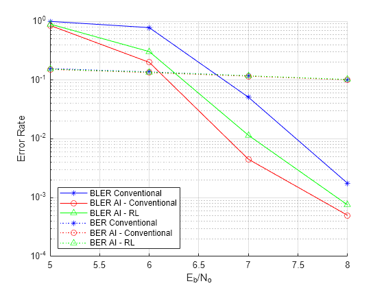
BLER curves show that the conventional autoencoder, which has full knowledge of the differentiable channel, outperforms the baseline system by about 0.7dB at 10% BLER. The RL-based autoencoder, which does not have the channel model, performs within 0.1 dB of the conventional autoencoder.

Discussions and Further Exploration

In this example, you implement a complex AI-based physical layer that uses custom training loops and custom loss functions. You simulate the system BLER performance over a link with a conventional LDPC outer code. To explore the system performance further, replace the channel model with more complex models such as comm.RayleighChannel, comm.RicianChannel, and comm.RayTracingChannel. Alternatively, use standards-based channels such as nrCDLChannel, nrTDLChannel, and nrHSTChannel. Vary the number of bits per symbol, bitsPerSymbol, codeword length, codewordLength, and number of blocks, $$N_{blk}$$.

For each new case, adjust the training parameters listed in the Training Parameters section.

The ConventionalEndtoEndTrainingCommunicationsSystemExample script shows how to train the same network with a known channel model and back propagation.

References

[1] F. Ait Aoudia and J. Hoydis, “Model-Free Training of End-to-End Communication Systems,” in IEEE Journal on Selected Areas in Communications, vol. 37, no. 11, pp. 2503-2516, Nov. 2019, doi: 10.1109/JSAC.2019.2933891.

[2] S. Cammerer, F. A. Aoudia, S. Dörner, M. Stark, J. Hoydis and S. ten Brink, "Trainable Communication Systems: Concepts and Prototype," in IEEE Transactions on Communications, vol. 68, no. 9, pp. 5489-5503, Sept. 2020, doi: 10.1109/TCOMM.2020.3002915.

Related Topics

• Deep Learning in MATLAB