Design Fractional Delay FIR Filters
Fractional delay filters shift a digital sequence by a noninteger value by combining interpolation and resampling into a single convolution filter. This example shows you how to design and implement fractional delay FIR filters using tools available in DSP System Toolbox™.
Delay as a Convolution System
Integer Delays
Consider the delay of a digital signal, , where D is an integer. You can represent this operation as a convolution filter, , with a finite impulse response, . The corresponding transfer function is , and the frequency response is . Programmatically, you can implement such an integer delay filter using the following MATLAB® code.
% Create the FIR
D = 3; % Delay value
h = [zeros(1,D) 1]
h = 1×4

     0     0     0     1
Shift a sequence by filtering it through the FIR h. The zeros at the beginning of the output signify the initial condition that is intrinsic to such filters.
x = (1:10)';
dfir = dsp.FIRFilter(h);
y = dfir(x)'
y = 1×10

     0     0     0     1     2     3     4     5     6     7
Fractional Delays via D/A Interpolation
The delay of the sequenceis undefined when D is not an integer. To make such fractional delays sensible and to sample the output on the continuum, you need to add an intermediate D/A interpolation stage. That is, , where denotes some D/A interpolation of the input sequence . can depend on n, and can represent an underlying analog signal model from which you sampled the sequence . This strategy is used in other resampling problems such as rate conversion.
This example features fractional delay filters using two interpolation models from DSP Systems Toolbox.
Sinc-based interpolation model: Use bandlimited reconstruction for .
Lagrange-based interpolation model: Use polynomial reconstruction for .
Bandlimited Fractional Delay Filters
The Shannon-Whittaker interpolation formula models bandlimited signals. That is, the intermediate D/A conversion is a bandlimited reconstruction of the input sequence. For a delay value, D, you can represent the fractional delay , which uses the same for every n, as a convolution filter. This filter is called the ideal bandlimited fractional delay filter, and its impulse response is
.
The corresponding frequency response (that is, DTFT) is given by .
Causal FIR Approximation of Ideal Bandlimited Shift Filter
The ideal sinc-shift filter described in the previous section is an allpass filter (), but it has an infinite and noncausal impulse response . You cannot represent the filter as a vector in MATLAB but can instead represent it as a function of index k.
% Ideal Filter sequence
D = 0.4;
hIdeal = @(k) sinc(k-D);
For practical and computational purposes, you can truncate the ideal filter on a finite index window, at the cost of some bandwidth loss. For a target delay value of and a desired length of N, the window of indices satisfying is symmetric about and captures the main lobe of the ideal filter. For where and is an integer, the explicit window indices are. The integer is referred to as the integer latency, and you can select it arbitrarily. To make the FIR causal, set , so the index window is . This code depicts the rationale behind the causal FIR approximation.
% FIR approximation with causal shift
N = 6;
idxWindow = (-floor((N-1)/2):floor(N/2))';
i0 = -idxWindow(1); % Causal latency
hApprox = hIdeal(idxWindow);
plot_causal_fir("sinc",D,N,i0,hApprox,hIdeal);
![Figure contains 2 axes objects. Axes object 1 with title sinc-based Fractional Delay Non-Causal FIR, Truncated on [-2:3], xlabel Sample Index, ylabel FIR Coefficients contains 6 objects of type stem, patch, scatter, line, constantline. These objects represent Truncated FIR, Anti-Causal Indices, Causal Indices, Ideal Filter. Axes object 2 with title Causal Shift of sinc-based Fractional Delay FIR, Truncated on [0:5], xlabel Sample Index, ylabel FIR Coefficients contains 3 objects of type stem, patch, constantline. These objects represent Truncated Causal FIR, All Causal Indices.](../../examples/dsp/win64/DesignOfFractionalDelayFiltersExample_01.png)
Truncating a sinc filter causes a ripple in the frequency response, which you can address by applying weights (such as Kaiser or Hamming) to the FIR coefficients.
The resulting FIR approximation model of the ideal bandlimited fractional delay filter is represented as follows.
You can design such a filter using the designFracDelayFIR function and the dsp.VariableFractionalDelay System object™ with the interpolation method set to 'FIR'. The function and the System object use Kaiser window weights.
Lagrange-Based Fractional Delay Filters
Lagrange-based fractional delay filters use polynomial fitting on a moving window of input samples. That is, is a polynomial of the fixed degree K. Like the sinc-based delay filters, you can formulate Lagrange-based delay filters as causal FIR convolution () of the length N = K+1 supported on the index window. As in the sinc-based model, apply the causal latency . Given a fractional delay , you can obtain the FIR coefficients of the (causal shifted) Lagrange delay filter by solving a system of linear equations. These equations describe a standard Lagrange polynomial fitting problem.
are the enumerated indices of the sample window. Use this code to implement the filter.
% Filter parameters
FD = 0.4;
K = 7;    % Polynomial degree
N = K+1;  % FIR Length
idxWindow = (-floor((N-1)/2):floor(N/2))';

% Define and solve Lagrange interpolation equations
V = idxWindow.^(0:K); % Vandermonde structure
C = FD.^(0:K);

hLagrange = C/V;  % Solve for the coefficients
i0 = -idxWindow(1); % Causal latency
plot_causal_fir("Lagrange",FD,N,i0,hLagrange);
![Figure contains 2 axes objects. Axes object 1 with title Lagrange-based Fractional Delay Non-Causal FIR, Supported on [-3:4], xlabel Sample Index, ylabel FIR Coefficients contains 4 objects of type stem, patch, constantline. These objects represent FIR, Anti-Causal Indices, Causal Indices. Axes object 2 with title Causal Shift of Lagrange-based Fractional Delay FIR, Supported on [0:7], xlabel Sample Index, ylabel FIR Coefficients contains 3 objects of type stem, patch, constantline. These objects represent Causal FIR, All Causal Indices.](../../examples/dsp/win64/DesignOfFractionalDelayFiltersExample_02.png)
You can implement this model as a direct-form FIR filter if the delay value FD is fixed, or using a Farrow structure if the delay value varies. For more information on implementing Lagrange interpolation using the Farrow mode, see the Design And Implement Lagrange-Based Delay Filters section in this example.
Design And Implement Sinc-Based Fractional Delay FIR Filters
This section shows you how to design and implement sinc-based fractional delay filters.
designFracDelayFIR Function in Length-Based Design Mode
Use the designFracDelayFIR function to design a fractional delay FIR filter with delay FD and length N. This function provides a simple interface to design such filters.
FD = 0.32381;
N = 10;
h = designFracDelayFIR(FD,N)
h = 1×10

    0.0046   -0.0221    0.0635   -0.1664    0.8198    0.3926   -0.1314    0.0552   -0.0200    0.0042
Implement the filter using the dsp.FIRFilter System object.
% Create an FIR filter object
fdfir = dsp.FIRFilter(h);
Delay a signal by filtering it through the designed filter.
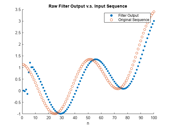
% Generate some input
n = (1:100)';
x = gen_input_signal(n);

% Filter the input signal
y = fdfir(x);
plot_sequences(n,x, n,y);
legend('Filter Output','Original Sequence')
title('Raw Filter Output v.s. Input Sequence')
The actual filter delay is not , but because of the causal integer latency . The designFracDelayFIR function returns the latency as the second output argument.
[h,i0] = designFracDelayFIR(FD,N);
The overall delay is merely the sum of the desired fractional delay and the incurred integer latency.
Dtotal = i0+FD
Dtotal =
4.3238
This total delay is also the group delay of the FIR filter at low frequencies. Verify that by using the outputDelay function.
[Doutput,~,~] = fdfir.outputDelay(Fc=0)
Doutput =
4.3238
Shift the plot of the input sequence by the total delay to align the filter output with the expected result.
plot_sequences(n+Dtotal,x, n,y);
legend('Filter Output','Input Sequence (shifted by FD+i0)')
title('Filter Output v.s. Time Adjusted Input Sequence')
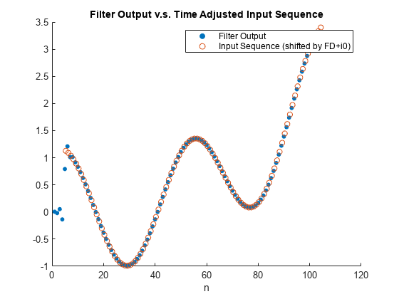
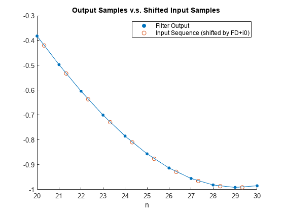
The shifted input markers located at generally do not coincide with the output samples markers , because falls on noninteger values on the x-axis, whereas n is an integer. The shifted input samples fall approximately on a line connecting the two consecutive output samples.
plot_sequences(n+i0+FD,x, n,y,'with line');
legend('Filter Output','Input Sequence (shifted by FD+i0)')
title('Output Samples v.s. Shifted Input Samples ')
xlim([20,30])
dsp.VariableFractionalDelay System Object in 'FIR' Mode
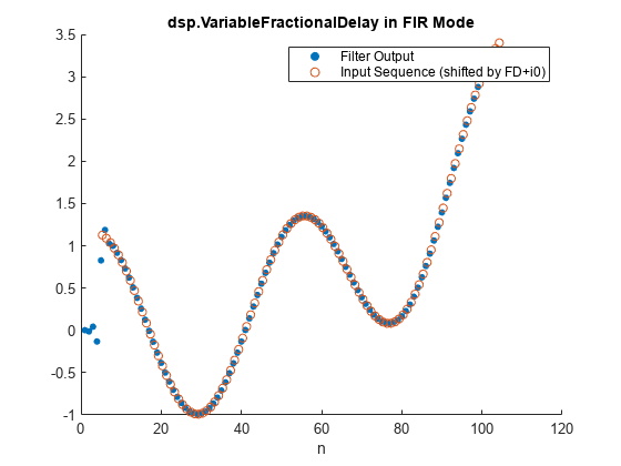
You can also design sinc-based delay filters using the dsp.VariableFractionalDelay System object and by setting its interpolation method property to 'FIR'. Begin by creating an instance of the System object. The FIR length is always even, and you can specify it in the FilterHalfLength property.
vfd_fir = dsp.VariableFractionalDelay(InterpolationMethod = 'FIR', FilterHalfLength = N/2);
i0_vfd_fir = vfd_fir.FilterHalfLength;    % Integer latency
Pass the desired fractional delay as the second input argument to the object call. Make sure that the delay value you specify includes the integer latency.
y = vfd_fir(x,i0+FD);
release(vfd_fir)
plot_sequences(n+i0+FD,x, n,y);
legend('Filter Output','Input Sequence (shifted by FD+i0)')
title('dsp.VariableFractionalDelay in FIR Mode')
Compare designFracDelayFIR and dsp.VariableFractionalDelay in 'FIR' Mode
Both designFracDelayFIR and dsp.VariableFractionalDelay in 'FIR' mode provide sinc-based fractional delay filters, but their implementations are different.
The
dsp.VariableFractionalDelaySystem Object approximates the delay value by a rational number up to some tolerance, and then samples the fractional delay as the k-th phase of a (long) interpolation filter of length L. This requires more memory, and yields less accurate delay.By contrast, the
designFracDelayFIR functiongenerates the FIR coefficients directly, rather than sampling them from a longer FIR. This allows the function to provide a precise fractional delay value, and costs less memory.The
designFracDelayFIRfunction has a simple interface that returns FIR coefficients, and leaves the filter implementation to the user. The interface of thedsp.VariableFractionalDelaySystem object allows you to both design and implement the filter.
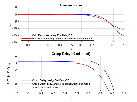
Use the designFractionalDelayFIR function over the dsp.VariableFractionalDelay System Object in the 'FIR' mode for its simplicity, better performance, and efficiency. This figure shows that the filter designed using dsp.VariableFractionalDelay has a shorter bandwidth, and its group delay is off by ~0.02 from the nominal value.
% Obtain the FIR coefficients from the dsp.VariableFractionalDelay object
h_vfd_fir = vfd_fir([1;zeros(31,1)],i0_vfd_fir+FD);
release(vfd_fir);
plot_freq_and_gd(h,i0,[],"designFracDelayFIR", h_vfd_fir,i0_vfd_fir,[],"dsp.VariableFractionalDelay FIR mode");
hold on;
yline(FD,'DisplayName','Target Fractional Delay');
ylim([-0.1,0.4])
Design and Implement Lagrange-Based Delay Filters
Lagrange-based fractional delay filters are computationally cheap and you can implement them efficiently using the Farrow structure. The Farrow filter is a special type of FIR filter that you can implement using only elementary algebraic operations, such as scalar additions and multiplications. Unlike the sinc-based designs, Farrow filters do not require specialized functions (such as sinc or Bessel) to compute the delay FIR coefficients. This makes Farrow fractional delay filters particularly simple to implement on a basic hardware.
The downside of Lagrange-based delay filters is that they are limited to lower orders, due to the highly unstable nature of higher order polynomial approximations. Using this method usually results in a lower bandwidth filter, as compared to a sinc-based filter.
Another type of a computationally-cheap fractional delay filter is the Thiran filter. See thiran (Control System Toolbox) for more information.
The System Object dsp.VariableFractionalDelay in 'Farrow' mode
Use the dsp.VariableFractionalDelay System object in the 'Farrow' mode to create and implement Farrow delay filters. Begin by creating an instance of the System object:
vfd = dsp.VariableFractionalDelay(InterpolationMethod = 'Farrow', FilterLength = 8);
i0var = floor(vfd.FilterLength/2) % Integer latency of the filter
i0var =
4
Apply the object to an input signal and plot the result.
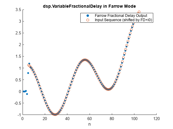
y = vfd(x,i0var+FD);
plot_sequences(n+i0var+FD,x, n,y);
legend('Farrow Fractional Delay Output','Input Sequence (shifted by FD+i0)')
title('dsp.VariableFractionalDelay in Farrow Mode')
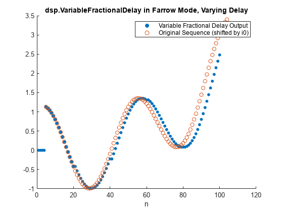
You can also vary the fractional delay values. This code operates on frames of 20 samples while increasing the delay value with each frame. Note the increase of the delay in the output graph corresponding to the changes in the delay values.
release(vfd)
FDs = i0var+5*(0:0.2:0.8); % Fractional delays vector
xsource = dsp.SignalSource(x,20);
ysink = dsp.AsyncBuffer;
for FD=FDs
    xk = xsource();
    yk = vfd(xk, FD);
    write(ysink,yk);
end
y = read(ysink);

plot_sequences(n+i0var,x, n,y);
legend('Variable Fractional Delay Output','Original Sequence (shifted by i0)')
title('dsp.VariableFractionalDelay in Farrow Mode, Varying Delay')
Bandwidth of FIR Fractional Delay Filters: Analysis and Design
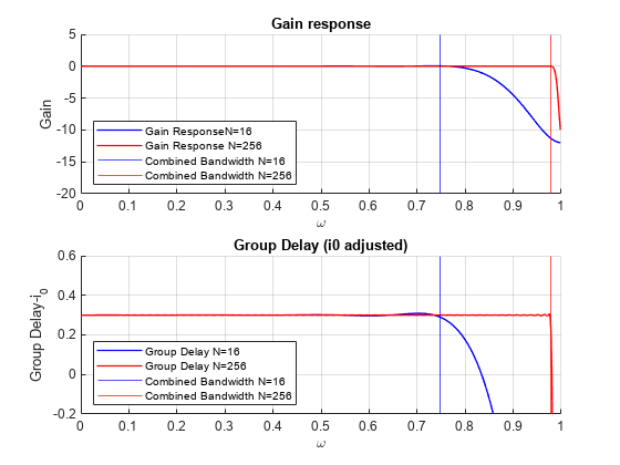
Longer filters provide better approximations of the ideal delay filter in terms of raw quadratic norms. However, practically a more meaningful metric, such as the bandwidth is needed. The function designFracDelayFIR measures combined bandwidth, which is defined as the frequency range in which both the gain and the group delay are within 1% of their nominal values. You can obtain the measured combined bandwidth from the designFracDelayFIR function. Design two FIR fractional delay filters of length 16 and 256. Plot the gain and group delay of the two filters. As expected, the longer filter (in red in the plot) has a significantly higher combined bandwidth.
FD = 0.3;
N1 = 16;
N2 = 256;
[h1,i1,bw1] = designFracDelayFIR(FD, N1);
[h2,i2,bw2] = designFracDelayFIR(FD, N2);

plot_freq_and_gd(h1,i1,bw1,"N="+num2str(N1), h2,i2,bw2,"N="+num2str(N2));
ylim([-0.2,0.6])
designFracDelayFIR Function in Bandwidth Design Mode
In the bandwidth design mode, the designFracDelayFIR function can determine the required filter length for a given bandwidth. Specify the delay value and the desired target bandwidth as inputs to the function, and the function finds the appropriate filter length.
FD = 0.3;
bwLower = 0.9; % Target bandwidth lower limit
[h,i0fixed,bw] = designFracDelayFIR(FD,bwLower);
fdfir = dsp.FIRFilter(h);
info(fdfir)
ans = 6×35 char array
'Discrete-Time FIR Filter (real) '
'------------------------------- '
'Filter Structure : Direct-Form FIR'
'Filter Length : 52 '
'Stable : Yes '
'Linear Phase : No '
bwLower is merely a lower bound for the combined bandwidth. The function returns a filter whose combined bandwidth is at least the value specified in bwLower.
Distortion in High Bandwidth Signals
In this section, you compare the performance of the two design points (long sinc v.s. short Lagrange) with a high bandwidth input. The filter you designed using the dsp.VariableFractionalDelay System object in the previous section is an 8-degree Farrow structure, effectively an FIR of length 9. The filter you designed using the designFracDelayFIR function, with FD = 0.3 and bwLower = 0.9, has a length of 52 samples. Plot the two FIR frequency responses on the same graph to demonstrate the bandwidth difference between the two.
release(vfd);
hvar = vfd([1;zeros(31,1)],i0var+FD);
plot_freq_and_gd(h,i0fixed,bw,"Sinc-based", hvar,i0var,[],"Farrow");
ylim([-0.2,0.6])
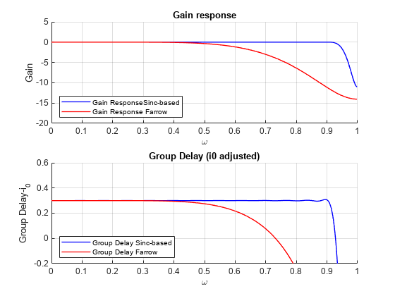
Apply the two filters to a high-bandwidth signal, Plot the time (top row) and frequency (bottom row) response of the two signals to compare the performance of the two filters (sinc on the left and Farrow on the right).
n=(1:80)';
x = high_bw_signal(n);

y1 = fdfir(x);
y2 = vfd(x,i0var+FD);

plot_signal_comparison(n,x,y1,y2,h,hvar,i0fixed,i0var,FD);

The results are as expected:
The longer sinc filter has a higher bandwidth. The shorter Farrow filter has a lower bandwidth.
Signal distortion is virtually nonexistent in the longer sinc filter, but easily noticeable in the shorter Farrow filter.
Higher accuracy comes at the expense of longer latency: approximately 25 samples v.s. only 4 in the shorter filter.
dsp.VariableFractionalDelay or designFracDelayFIR ?
You can choose between the dsp.VariableFractionalDelay System object and the designFracDelayFIR function based on the filter requirements and the target platform.
For a high bandwidth and accurate group delay response, use the
designFracDelayFIRfunction. Keep in mind that this design process is more intensive computationally. Therefore, deploy the function on high-end hardware if you want to tune the delay values in real time. You can deploy it on low-end hardware if you fix the delay value and design the filter offline.For time-varying delay filters aimed at low-performance computational apparatus, use
dsp.VariableFractionalDelayin the'Farrow'mode.