Fault Detection and Localization in Three-Phase Power Transmission Using Deep Signal Anomaly Detector in Simulink

This example shows how to detect and localize faults in three-phase electrical power systems using the Deep Signal Anomaly Detector block in Simulink®. The Deep Signal Anomaly Detector block uses a trained LSTM autoencoder network to reconstruct the input signal and thresholds the loss of reconstruction to detect anomalies in input data. This example uses the deepSignalAnomalyDetector function in Signal Processing Toolbox to create and train the LSTM autoencoder to be used in the detector block. The Deep Signal Anomaly Detector block requires DSP System Toolbox and Deep Learning Toolbox.

The two most typical faults in three-phase power systems are open-circuit fault and short-circuit fault. Open circuit faults mainly occur because of common issues like failure in the phase of a circuit breaker or melting of conductor or fuse within one phase or more phases. Short-circuit faults occur when there is an abnormal connection of very low impedance between different phase lines or between a phase line and earth. These faults are mainly due to failure of insulation on conductors. This example focuses on the detection of short-circuit faults.

Short-circuit faults can be divided into the following categories:

• L-G fault : This type of fault occurs when one of the phases (A, B or C) is shorted with the ground.

• L-L fault : This type of fault occurs when two of the phases are shorted with each other.

• L-L-G fault: This type of fault occurs when two of the phases are shorted with each other and also the ground.

• L-L-L fault: This type of fault occurs when all the three phases are shorted with each other.

• L-L-L-G fault: This type of fault occurs when all the three phases are shorted with each other and also the ground.

Among these faults, L-L-L and L-L-L-G faults are considered symmetric faults since they affect all the phases equally. L-G, L-L, L-L-G faults are considered asymmetric faults.

Modeling three-phase power transmission system

This example uses components from Simscape™ Electrical™ to simulate a basic electrical power system and introduce faults. For more details on modeling three-phase electrical systems using components from Simscape Electrical, refer to Build and Simulate Composite and Expanded Three-Phase Models (Simscape Electrical).

Open and examine the Simulink model PowerTransmissionModel which is designed to model the power transmission system.

powersysModel = "PowerTransmissionModel.slx";
open_system(powersysModel);

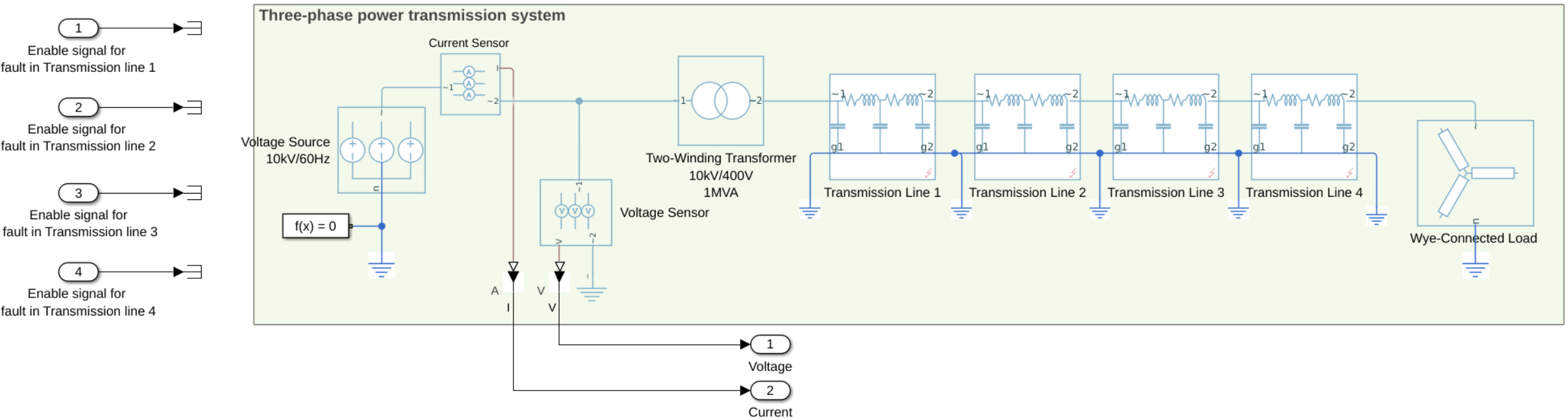
Use a Voltage Source (Three-Phase) (Simscape Electrical) block to model the power source. Configure the source block to have a phase-to-phase RMS voltage of 10kV at frequency 60Hz. Use a Current Sensor (Three-Phase) (Simscape Electrical) block and Phase Voltage Sensor (Three-Phase) (Simscape Electrical) block to measure the three-phase currents and voltages respectively near the source. These measured voltages and currents are utilized in subsequent sections of the example as the input features for training the autoencoder network and detecting anomalies.

Use a Two-Winding Transformer (Three-Phase) (Simscape Electrical) block to implement a transformer to step down the source voltage (10kV/400V). Set the connection type of both windings to "Wye with grounded neutral" to ensure that faults in one phase do not impact the voltage and current in the other phases. Model a transmission line of length 400m at the secondary winding of the transformer using four Transmission Line (Three-Phase) (Simscape Electrical) blocks. These transmission lines are connected in series and each have a length of 100m. To represent the load at the end of the transmission line, connect a Wye-Connected Load (Simscape Electrical) block.

The four Transmission Line blocks have been configured to have four different short-circuit faults:

• Transmission line 1: L-G fault in Phase A

• Transmission line 2: L-L fault in Phases A,B

• Transmission line 3: L-L-G fault in Phases B,C

• Transmission line 4: L-L-L fault in Phases A,B,C

These faults can be enabled with the help of four enable signals using the Inport blocks on the left side of the model. For more details on modeling faults in Simulink, see Get Started with Simulink Fault Analyzer (Simulink Fault Analyzer). In this example, we create conditional faults for the Transmission Line blocks. A fault is introduced in the transmission line when the value of the corresponding enable signal is greater than 0 and the fault turns off if the enable signal is equal to 0. For more details on the use of conditionals to introduce faults, refer to Create and Manage Conditionals (Simscape). This example considers intermittent faults, where each fault exists only for a short time interval during the simulation.

The PowerTransmissionModel model is used in subsequent sections as a Model References (Simulink) to simulate the power transmission system.

Generate training data

Open the Simulink model TrainingModel. Use this model to generate the training data for the autoencoder.

close_system(powersysModel,0);
trainModel = "TrainingModel.slx";
open_system(trainModel);

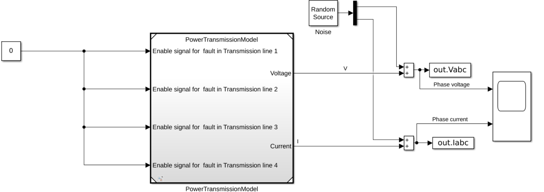
The deep learning network for anomaly detection needs to be trained using "normal" training that does not contain any anomalies. To emulate the three-phase power system, this model utilizes the PowerTransmissionModel introduced in the earlier section, as a Model Reference. To simulate the system without introducing any faults, set the enable signals for each of the four faults to 0 using a Constant (Simulink) block. Add Gaussian noise to the voltage and current measurements to make the autoencoder model more robust.

Simulate the model to generate the training data.

out = sim(trainModel);
close_system(trainModel,0);

The three-phase currents and voltages are used as input features to train the network. Since the ranges of voltages and currents can be different, normalize their values using the respective values of standard deviation.

Vabc = out.Vabc; 
Iabc = out.Iabc;

stdV = std(Vabc(:));
stdI = std(Iabc(:));

% Normalize voltages and currents
Vabc = Vabc/stdV;
Iabc = Iabc/stdI;

% Combine normalized voltage and currents
VInorm = [Vabc Iabc];

Part 1: Detect fault in three-phase transmission line

This section shows how to detect the occurrence of a fault in three-phase power line, without explicitly identifying the specific lines in which the fault occurs.

Create and train the LSTM autoencoder

Use the function deepSignalAnomalyDetector to create an LSTM autoencoder of type deepSignalAnomalyDetectorLSTM. Set the number of channels to 6 considering the 3 values of voltages and currents. Use a single layer each in the encoder and decoder, with 32 hidden units in the layer.

Set the value of SequenceLength to 64 in trainingOptions (Deep Learning Toolbox). Note that setting an excessively high value for SequenceLength can lead the network to converge to a local minimum while training, leading to the network consistently predicting the mean value of the signal.

When a short-circuit fault occurs, the line voltages and currents are expected to be significantly different from the training data, and in turn the reconstruction loss is also expected to be much higher when a fault occurs. Hence you can adjust the value of threshold to a value significantly higher than the maximum loss observed in the training data. To configure the threshold value for fault detection as twice the maximum value of loss observed in the training data, set the ThresholdMethod property of the deepSignalAnomalyDetectorLSTM object to max, and the ThresholdParameter property to 2.

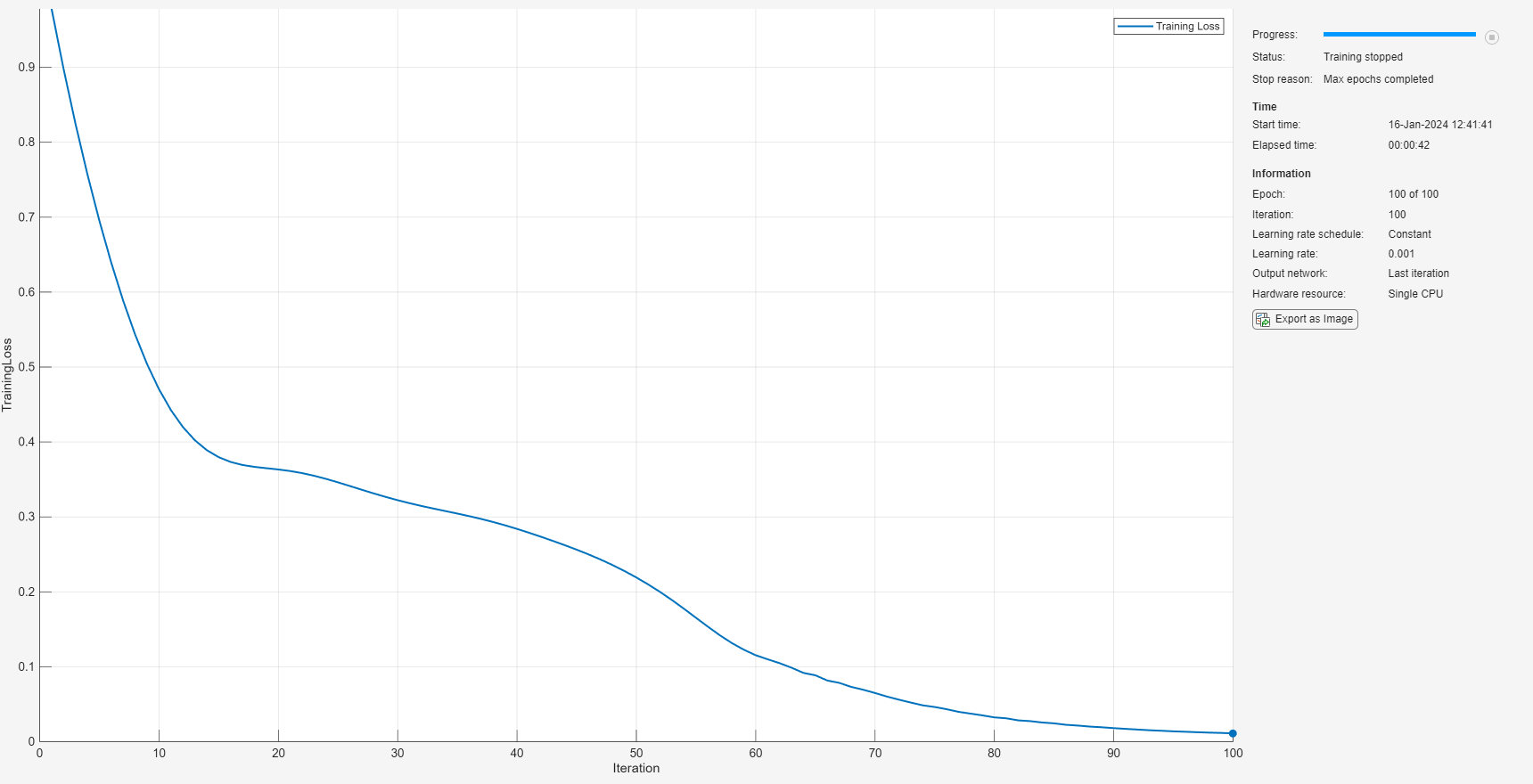
Train the network for 100 epochs. The training time is approximately 30 seconds on a Windows machine with an NVIDIA Quadro P620 GPU.

detector = deepSignalAnomalyDetector(6,"lstm",EncoderHiddenUnits=32 ,...
    DecoderHiddenUnits=32, WindowLength=50,ThresholdMethod="max",ThresholdParameter=2);

% Set training options
sequenceLength = 64;
options = trainingOptions("adam", ...
    MaxEpochs=100, ...
    SequenceLength=sequenceLength,...
    Plots="training-progress");

% Train the detector
trainNow = true;
if trainNow
    trainDetector(detector,VInorm,options);
end

    Iteration    Epoch    TimeElapsed    LearnRate    TrainingLoss
    _________    _____    ___________    _________    ____________
            1        1       00:00:06        0.001         0.97795
           50       50       00:00:30        0.001         0.21914
          100      100       00:00:41        0.001        0.011119
Training stopped: Max epochs completed

Computing threshold...
Threshold computation completed.

Save the trained network and detection parameters of the trained detector to a MAT-file.

if trainNow
    saveModel(detector,"threePhaseFaultDetector.mat");
end

Fault detection in Simulink

Open and examine the Simulink model FaultDetectionModel. This model simulates a three-phase power transmission system with short-circuit faults and detects these faults using the Deep Signal Anomaly Detector block by making use of the MAT-file generated in the previous step.

detectionModel = "FaultDetectionModel";
open_system(detectionModel);

Fault generation

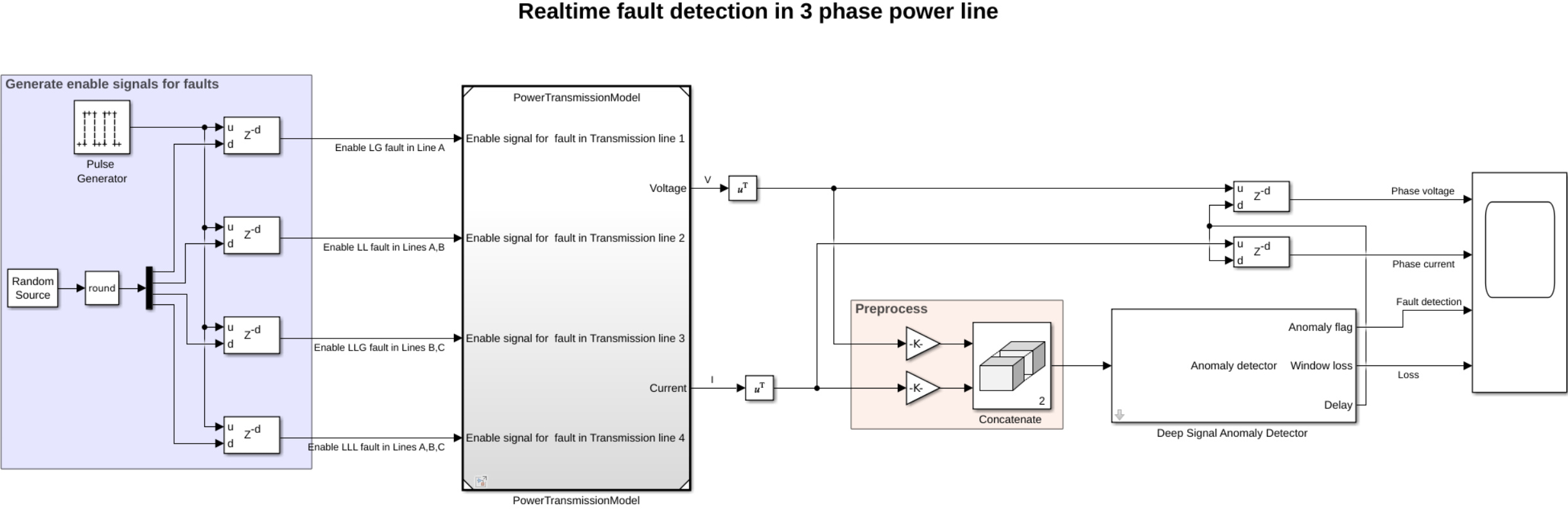
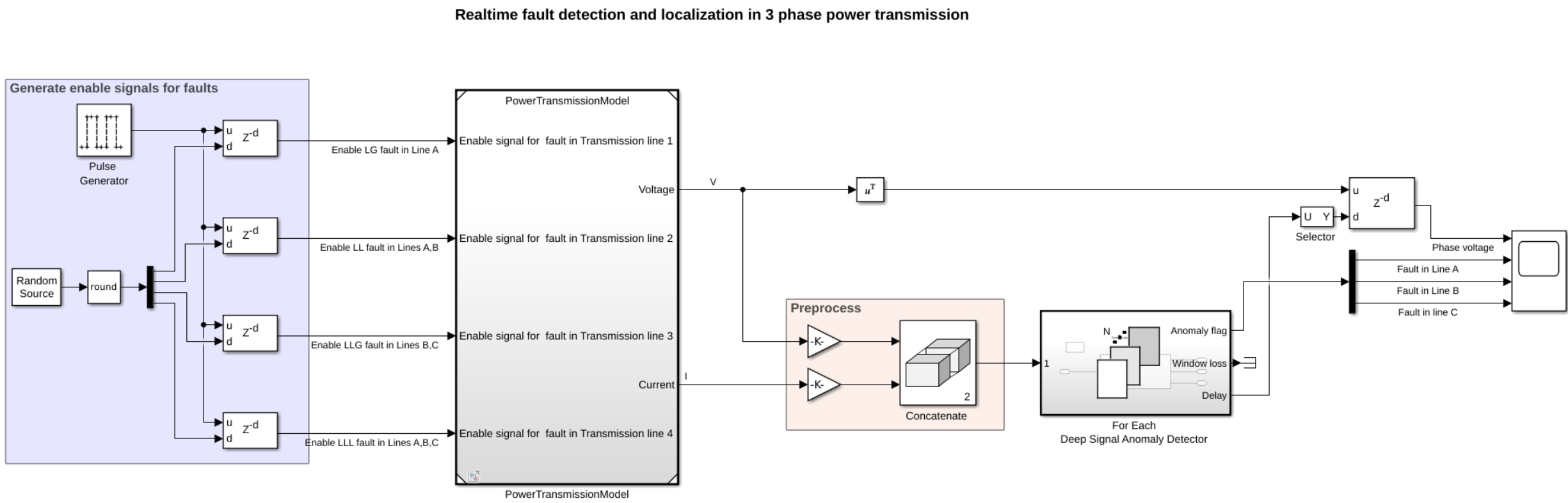
Similar to the training model, this model utilizes PowerTransmissionModel as a Model Reference. The "Generate enable signals for faults" area highlighted in blue creates enable signals for the faults in the four regions of the transmission line. Four intermittent faults are introduced in the transmission line in this example:

• L-G fault in a random interval of duration 0.1 second between simulation times 0 and 0.5 seconds in Phase A

• L-L fault in a random interval of duration 0.1 second between simulation times 0.5 and 1 seconds in Phases A,B

• L-L-G fault in a random interval of duration 0.1 second between simulation times 1 and 1.5 seconds in Phases B,C

• L-L-L fault in a random interval of duration 0.1 second between simulation times 1.5 and 2 seconds in Phases A,B,C

The Pulse Generator (Simulink) block generates enable signals for faults, while the Random Source block coupled with the Delay (Simulink) block randomizes the occurrence of the fault within specified intervals to generate the enable signals.

Anomaly detection

The Preprocess area highlighted in red normalizes the voltage and current values by their respective standard deviations calculated previously. These normalized values are concatenated to generate input features of size 6 and features are passed to the Deep Signal Anomaly Detector block. On the block, check that the Detector MAT-file path parameter is set to threePhaseFaultDetector.mat, which is the name of the MAT-file generated in the earlier section. In the block dialog, you can see the values of the post-processing parameters such as Window length, Threshold etc. that are read from the MAT-file. You can change these values to be used by the block by setting the Parameters for post-processing parameter to Specify on dialog and specifying the parameter values individually.

Two Delay blocks are employed to delay the measured voltage and current signals and align them with the outputs of the Deep Signal Anomaly Detector block. Note that when setting the Delay length parameter to "input port", the Delay length upper limit parameter must be set to a value higher than the value of delay length provided from the input port.

Simulate the model.

sim(detectionModel);

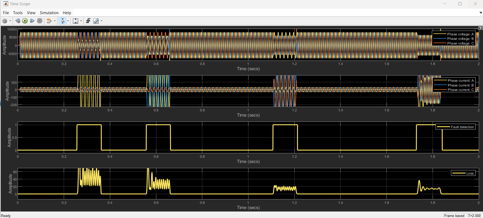
On the Time Scope you can see the delayed three-phase voltage and current signals, fault detection and estimated loss.

Note that at the start of the simulation, small regions of anomaly may be detected before Deep Signal Anomaly Detector block processes the first samples of the voltage and current measurements. This is due to the delay introduced by the block, resulting in the initial input samples being zeros.

Observe on the scope that the Deep Signal Anomaly Detector block accurately detects the 4 faults introduced in the transmission line. These fault regions exhibit significantly higher loss values compared to the regions without faults.

For example, you can see a fault of duration 0.1 seconds has been detected within the time interval (0,0.5) seconds. This corresponds to the L-G fault that was added in line A. This is reflected in the increased line current and reduced line voltage in Phase A. The line voltages and line currents in other phases are unchanged.

In the time interval (1,1.5) seconds, a fault of duration 0.1 seconds has been detected. This corresponds to the L-L-G fault that was added in lines B,C. This is reflected in the increased line currents in phases and reduced line voltages in phases B,C.

Part 2 : Localize faults in three-phase transmission line

This section shows how to detect and localize faults in a three-phase power line. In addition to fault detection, it also identifies the specific phases affected by the fault.

Create and train the LSTM autoencoder

To localize faults, analyze the voltage and current features of each individual phase independently. Utilize three separate anomaly detector units to identify faults in the respective phases. In this scenario, each phase's anomaly detector processes input data with two features: voltage and current readings in the respective phase.

Since the example handles a balanced three-phase system, a single deepSignalAnomalyDetectorLSTM object can be trained using voltage and current data from all the three phases. Three instances of this trained detector can then be employed for fault localization in each phase.

Combine the data from all three phases to a cell array. As previously mentioned, differentiating between the three phases is not necessary during the training stage due to the balanced nature of the three-phase system being considered.

VINormCell = {VInorm(:,[1,4]), VInorm(:,[2,5]), VInorm(:,[3,6])};

Create the LSTM autoencoder object using the deepSignalAnomalyDetector function. Set the number of channels to 2, as the input data includes one value of voltage and current each. Use the same settings in Part 1 for rest of the parameters.

Train the detector for 50 epochs and save the parameters of the trained detector to a MAT-file.

localizer = deepSignalAnomalyDetector(2,"lstm",EncoderHiddenUnits=32 ,...
    DecoderHiddenUnits=32, WindowLength=50,ThresholdMethod="max",ThresholdParameter=2);

options.MaxEpochs = 50;
% Train the detector
if trainNow
    trainDetector(localizer,VINormCell,options);
end

    Iteration    Epoch    TimeElapsed    LearnRate    TrainingLoss
    _________    _____    ___________    _________    ____________
            1        1       00:00:00        0.001            1.07
           50       17       00:00:12        0.001         0.22268
          100       34       00:00:23        0.001        0.010782
          150       50       00:00:33        0.001       0.0045543
Training stopped: Max epochs completed

Computing threshold...
Threshold computation completed.

Save the trained network and detection parameters of the trained detector to a MAT-file.

if trainNow
    saveModel(localizer,"threePhaseFaultLocalizer.mat");
end

Fault detection and localization in Simulink

Open the Simulink model FaultLocalizationModel.

close_system(detectionModel,0);
localizationModel = "FaultLocalizationModel";
open_system(localizationModel);

This model uses the same setup as the model FaultDetectionModel discussed in Part 1 to create a three-phase power transmission system and introduce short-circuit faults.

The Preprocess area highlighted in red normalizes the voltage and current values by their respective standard deviations and concatenates the voltage and current values along each phase in a different row. The output of the Concatenate block is of size 3-by-2 where each row contains the voltage and current values in a different phase.

As mentioned earlier, three different anomaly detectors are required to detect anomalies in each line independently. Instead of creating three separate instances of the Deep Signal Anomaly Detector block, you can place the block inside a For Each Subsystem (Simulink). The For-Each subsystem enables you to perform the same computation over the elements of an input signal by applying the same operations to each element individually and independent from each other. For more information on how to use the For-Each subsystem, refer to the example Vectorizing a Scalar Algorithm with a For-Each Subsystem (Simulink).

Place the Deep Signal Anomaly Detector block inside a For Each subsystem. Set the Detector MAT-file path parameter of the block to threePhaseFaultLocalizer.mat, which is the name of the MAT-file generated in the earlier section.

Set the Partition Dimension parameter of theFor Each (Simulink) block to 1, corresponding to rows, since each row of the input contains the data corresponding to a different phase.

The For Each subsystem concatenates the Anomaly flags and Delay outputs from the three phases to vectors of size 3 each. Use a Demux (Simulink) block to separate the anomaly flags. Since the parameters of the anomaly detector employed for each phase is the same, the delay output for each of the phases is identical. Utilize a Selector (Simulink) block to select one of the 3 delay values and delay the measured voltage signals by this selected value using a Delay block. Visualize the three-phase voltage and the fault detection in the three phases using a Time Scope.

Simulate the model.

sim(localizationModel);

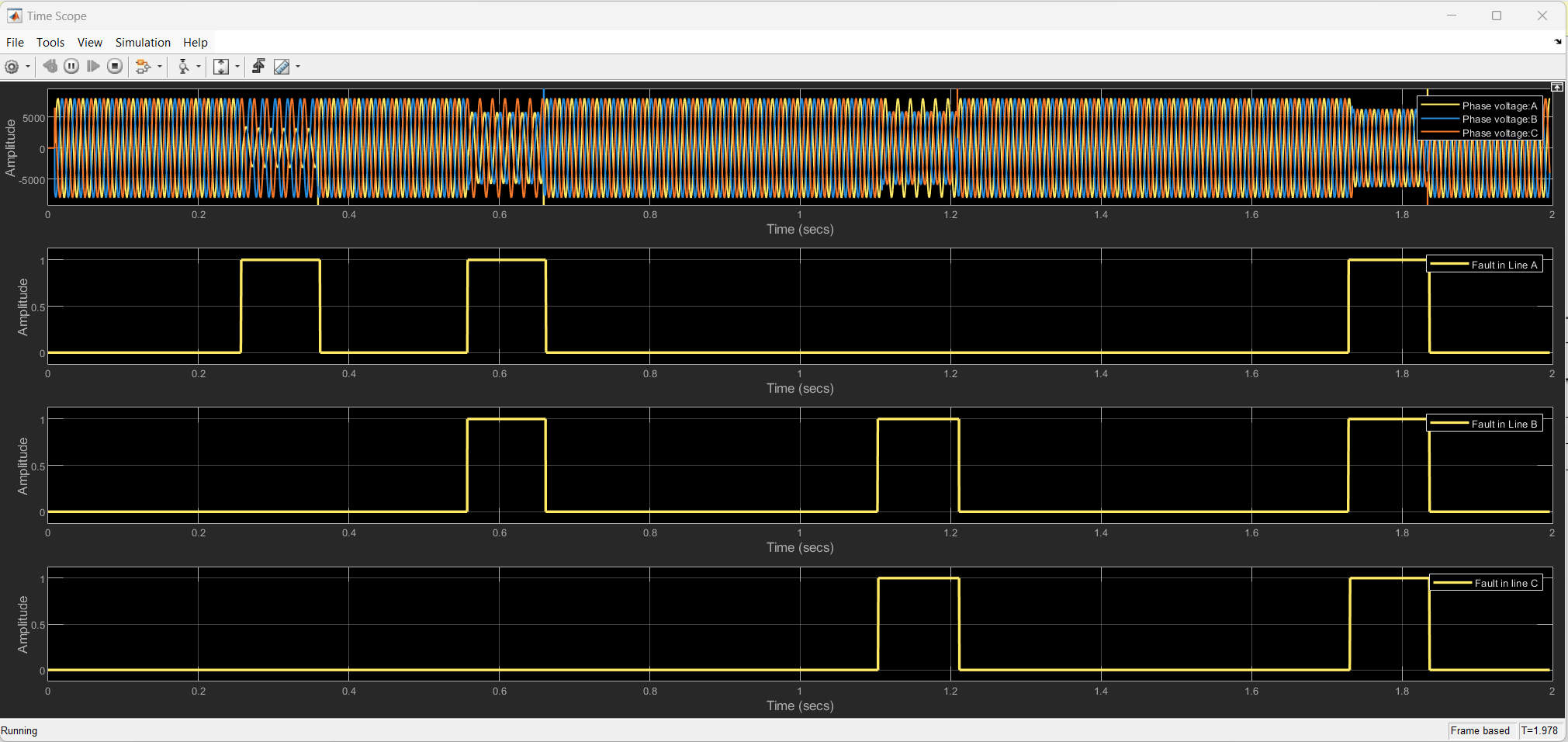
Observe the measured voltage in the three phases along with the fault detection on each of phases on the Time scope.

In the time interval (0,0.5) seconds, you can observe a fault of duration 0.1 seconds in line A corresponding to the L-G fault added in line A. In the interval (0.5, 1) seconds, you can observe a fault in the lines A,B corresponding to the L-L-G fault added in lines A,B. Similarly in the intervals (1, 1.5) seconds and (1.5, 2) seconds, you can observe faults in lines B,C and lines A,B,C corresponding to the L-L-G fault in lines B,C and L-L-L faults respectively.

close_system(localizationModel,0);

Summary

This example demonstrates the use of LSTM autoencoders to detect and localize short-circuit faults in three-phase power transmission systems. To detect the presence of a fault in the system without identifying the specific lines in which the fault occurs, train and employ a single anomaly detector by considering the voltage and current measurements across the phases as different features of the input data. To localize the fault, train the anomaly detector with two features (voltage, current), and employ a separate instance of the trained detector on each of the phases.