Infer Conditional Variances and Residuals
This example shows how to infer conditional variances from a fitted conditional variance model. Standardized residuals are computed using the inferred conditional variances to check the model fit.
Step 1. Load the data.
Load the Danish nominal stock return data included with the toolbox.
load Data_Danish
y = DataTable.RN;
T = length(y);

figure
plot(y)
xlim([0,T])
title('Danish Nominal Stock Returns')
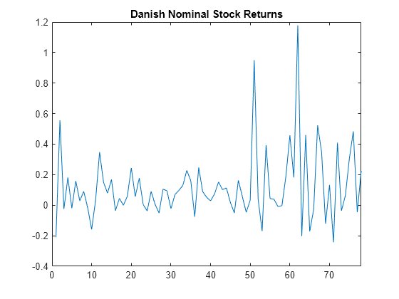
The return series appears to have a nonzero mean offset and volatility clustering.
Step 2. Fit an EGARCH(1,1) model.
Specify, and then fit an EGARCH(1,1) model to the nominal stock returns series. Include a mean offset, and assume a Gaussian innovation distribution.
Mdl = egarch('Offset',NaN','GARCHLags',1,...
    'ARCHLags',1,'LeverageLags',1);
EstMdl = estimate(Mdl,y);
    EGARCH(1,1) Conditional Variance Model with Offset (Gaussian Distribution):

                     Value       StandardError    TStatistic     PValue
                   __________    _____________    __________    _________

    Constant         -0.62723       0.74401        -0.84304        0.3992
    GARCH{1}          0.77419       0.23628          3.2766     0.0010508
    ARCH{1}           0.38636       0.37361          1.0341       0.30107
    Leverage{1}    -0.0024989       0.19222          -0.013       0.98963
    Offset            0.10325      0.037727          2.7368     0.0062047
Step 3. Infer the conditional variances.
Infer the conditional variances using the fitted model.
v = infer(EstMdl,y);

figure
plot(v)
xlim([0,T])
title('Inferred Conditional Variances')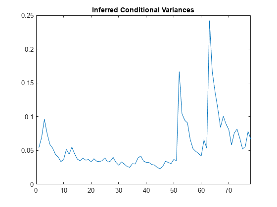
The inferred conditional variances show increased volatility at the end of the return series.
Step 4. Compute the standardized residuals.
Compute the standardized residuals for the model fit. Subtract the estimated mean offset, and divide by the square root of the conditional variance process.
res = (y-EstMdl.Offset)./sqrt(v);

figure
subplot(2,2,1)
plot(res)
xlim([0,T])
title('Standardized Residuals')

subplot(2,2,2)
histogram(res,10)

subplot(2,2,3)
autocorr(res)

subplot(2,2,4)
parcorr(res)
The standardized residuals exhibit no residual autocorrelation. There are a few residuals larger than expected for a Gaussian distribution, but the normality assumption is not unreasonable.