Nowcast GDP from Long Short-Term Memory Neural Network
R2026bThis example shows how to train a deep learning long short-term memory (LSTM) network to predict US gross domestic product (GDP).
Economic policy decisions require timely assessments of current conditions, yet key macroeconomic indicators such as GDP are published with substantial delays—typically four to six weeks after the end of the reference quarter. This publication lag creates an information void during which policymakers, businesses, and investors must form views about the present state of the economy without direct observation of the target variable. Nowcasting addresses this gap by exploiting the relationships between the target series and higher-frequency indicators that are more readily available. Monthly series such as industrial production, retail sales, and consumer sentiment—and increasingly, daily or weekly financial and survey data—provide valuable signals about ongoing economic activity well before official statistics appear.
To integrate these mixed-frequency data sources into coherent real-time estimates, a range of econometric frameworks has been developed, including dynamic factor models (DFMs), mixed-data sampling (MIDAS) regressions, and state-space approaches[1][2]. These methods optimally combine timely but partial indicators to infer the current state of GDP and other target variables, and have become central tools for central banks and policy institutions where real-time insight is crucial for effective oversight. More recently, advances in machine learning—particularly recurrent architectures such as long short-term memory (LSTM) networks—have opened new avenues for capturing complex temporal patterns within high-frequency economic data[20].
Import and Organize Economic Data
Import and preprocess historical observations of the indicators in this table from the Federal Reserve Bank of St. Louis.
Variable | Description | Frequency |
All employees, total non-farm[16] | Monthly | |
Unemployment rate[19] | Monthly | |
Average weekly hours of production and non-supervisory employees, total private[4] | Monthly | |
Industrial production, total index[15] | Monthly | |
Consumer price index (CPI) for all urban consumers, all items in US city average[7] | Monthly | |
Commercial and industrial loans, all commercial banks[5] | Monthly | |
New privately-owned housing units started, total units[13] | Monthly | |
Real GDP[11] | Quarterly | |
Fixed private investment[10] | Quarterly | |
GDP, implicit price deflator[12] | Quarterly | |
Non-farm business sector, hourly compensation for all workers[6] | Quarterly | |
Personal consumption expenditures (PCE)[17] | Monthly | |
PCE: chain-type price index[18] | Monthly | |
Real disposable personal income[8] | Monthly | |
Federal funds effective rate[9] | Monthly | |
10-year high quality market (HQM) corporate bond spot rate[14] | Monthly |
Connect to the Federal Reserve Economic Data (FRED®) server by using the fredrs (Datafeed Toolbox) function. The function requires an active FRED API key to authenticate requests and retrieve data. Replace its placeholder value of the apikey variable in this code block with your FRED API key.
apikey = "placeholder";
f = fredrs(apikey);
Fetch each indicator from the server and store the data in a timetable by using the local function localFetch (this function requires the Datafeed Toolbox™). Obtain observations from January 1, 2000 through December 31, 2024. Identify the frequency of each variable.
SeriesNames= ["PAYEMS" "UNRATE" "AWHNONAG" "INDPRO" "CPIAUCSL" ...
    "BUSLOANS" "HOUST" "GDPC1" "FPI" "GDPDEF" "COMPNFB" "PCE" "PCEPI" "DSPIC96" ...
    "FEDFUNDS" "HQMCB10YR"];
startdate = datetime(2000,1,1);
enddate = datetime(2024,12,31);

% Preallocate variables
isMonthly = true(numel(SeriesNames),1);
RawFredData  = timetable;

% Fetch data from FRED
for i = 1:numel(SeriesNames)
    TT = localFetch(f,SeriesNames(i));
    if days(diff(TT.Time(1:2))) < 40
        TT.Time = dateshift(TT.Time,"end","month");
    else
        TT.Time = dateshift(TT.Time,"end","quarter");
        isMonthly(i) = false;
    end
    RawFredData = synchronize(RawFredData,TT,"union");
end
Reorganize the data by performing the following actions:
Shift the dates to occur at the start of the month.
Position the quarterly variables at the end of the table, with the response variable
GDPC1being at the last position.
Ensure all observations are within the desired sampling range.
DataTbl = RawFredData;
DataTbl.Properties.DimensionNames(1) = "Date";
DataTbl.Date = dateshift(DataTbl.Date,"start","month");

varlist = SeriesNames(isMonthly);
varlist = upper([varlist SeriesNames(~isMonthly)]);

varlist(varlist == "GDPC1") = [];
varlist(end+1) = "GDPC1";

DataTbl = DataTbl(:,varlist);

range = [datetime(1999,1,1) datetime(2024,12,1)]; % 1999 first quarter to 2024 last quarter

ind = DataTbl.Properties.RowTimes>=range(1) & DataTbl.Properties.RowTimes<=range(2);
DataTbl = DataTbl(ind,:);
Synchronize and Stabilize Each Series
You must synchronize and stabilize mixed-frequency data before you fit it to a model.
Synchronize data by presenting all series on a unified monthly timeline and clearly indicating which months contain valid observations for each lower-frequency variable. A synchronized data set should have these characteristics:
The first column indicates the sampling months in ascending order.
Each subsequent column represents a different macroeconomic series, all expressed as seasonally adjusted growth rates at their available frequencies.
For lower frequency series (such as quarterly or yearly data), enter the values only in the final month of each period, e.g., December holds the value for annual data, and March, June, September, and December hold the values for quarterly data. Code all other months within the period as missing (
NaNfor numeric data).
This table illustrates a synchronized data set.
Date | Series1 | Series2 | Series3 | ... |
|---|---|---|---|---|
2024-01-01 | 0.01 | 0.002 |
| ... |
2024-02-01 | 0.012 | 0.001 |
| ... |
2024-03-01 | 0.009 | 0.002 | 0.004 | ... |
... | ... | ... | ... | ... |
2024-12-01 | 0.011 | 0.002 | 0.005 | ... |
Stabilize each series by expressing them as period-over-period growth rates. Specifically, compute the simple percent change between consecutive periods. This transformation standardizes the data, making the series stationary and more suitable for modeling by removing trends and scaling differences.
seriesID = varlist;
numMonth = sum(isMonthly);
numQuar = sum(~isMonthly);

% Monthly data
for j = varlist(1:numMonth)
    DataTbl.(j)(2:end) = DataTbl.(j)(2:end)./DataTbl.(j)(1:end-1)-1;
    DataTbl.(j)(1) = NaN;
end

% Quarterly data
for j = varlist(numMonth+1:end)
    DataTbl.(j)(6:3:end) = DataTbl.(j)(6:3:end)./DataTbl.(j)(3:3:end-3)-1;
    DataTbl.(j)(1:5) = NaN;
end
Build the LSTM Model
LSTM networks are well-suited for time series analysis because they effectively learn and remember long-term dependencies in sequential data. Unlike standard recurrent neural networks (RNNs), which struggle retaining information over long sequences due to the "vanishing gradient" problem, LSTMs employ a unique architecture featuring memory cells and gating mechanisms. These components enable LSTMs to selectively retain, update, or discard information as needed, which enables them to model intricate relationships and trends in economic indicators over time.
The LSTM model captures temporal dependencies and sequential patterns in macroeconomic time series data, which might improve the accuracy and timeliness of nowcast estimates. In this example, the goal of the LSTM model is to process sequences of multiple economic indicators and predict GDP over near-future time steps.
Create an LSTM model with the following characteristics:
The input, fully connected layer maps the input series to a 30-dimensional hidden state.
The network has two LSTM layers
The first LSTM layer maps the inputs to a 30-D hidden sequence.
The last LSTM layer collapses the 30-D sequence into a 16-D space.
At least 12 time steps must be in the input sequence.
Data normalization is off.
The final fully connected, linear layer produces the target nowcast.
latentDim = 30;
numLayers = 2;
numVars = size(DataTbl,2)-1;
targetLen = 1;

layers = [sequenceInputLayer(numVars,minlength=12,normalization="none",name="input")
    fullyConnectedLayer(30,Name="FC1")
    repmat(lstmLayer(latentDim,OutputMode="sequence"),numLayers-1,1)
    lstmLayer(16,OutputMode="last")
    fullyConnectedLayer(targetLen,Name="Output")
    ];

analyzeNetwork(layers)
Apply Vintage Analysis to Nowcasting Model
A key nowcasting challenge is that economic data is published on different schedules. This staggered data availability is characterized by periods where some indicators are available while others are not, which can impact estimation routines, forecasting, and model performance evaluation. In addition to the missing information, some high frequency observations are not published at the same time as others, which causes a "jagged-edge" at the end of the sample, where fewer observations are available. To realistically assess the performance of a nowcasting model, simulate staggered data and a jagged-edge by applying the data vintages process. Such simulations reflect the practical constraints faced by forecasters who must forecast using incomplete data; you can robustly evaluate models that include data vintage information because the process does not introduce future data revisions or hindsight bias.
A vintage analysis for nowcasting model evaluation follows these general steps:
Choose a historical date to nowcast. Call this date the target date. Reserve a variable containing the GDP during the test dates for comparison with the nowcasts.
Choose a number of months around the target date to simulate times when information is yet to be published for the chosen monthly series and quarterly series. Call these dates the vintage dates. In this example, the vintages dates are:
Two months before the target date. This vintage date represents the information landscape two months before the target, when many indicators for the period are not yet available.
One month before the target date.
The month of the target date.
One month after the target date.
Two months after the target date. At this point, the most relevant economic indicators for the target period have been published.
Choose several monthly series to have the same missing-observations pattern as the quarterly series.
Create two 3-D tensors of data, one tensor contains the GDP and the other tensor contains all other series, where each page contains a year of data, and successive pages shift forward by a month. Call the tensors the training data and target training data.
Train the LSTM to the tensor of training data through to three months before the target date to ensure the model is not trained on future observations. This trained model is the base model used to update the missing information.
Create a data set containing all observations to the target date. For the chosen monthly series and quarterly series and for each vintage date, fill the missing months from the end of the series with the associated training data means, to avoid data leakage and look-ahead bias, except for the GDP. Call these data sets the vintage data sets.
Obtain predictions for the GDP from the trained model for each vintage data set at the end of the data only.
Compare the vintage estimates with the actual observations.
Consider nowcasting GDPC1 monthly from the 2022Q3 through 2024Q4. Create a vector of those target quarters and a vector of the number of months ahead and behind each quarter to nowcast for the vintage analysis. Create the hold out sample from the target dates.
series = "GDPC1";
idx_GDP = find(strcmpi(series,seriesID));
testDateRange = [datetime(2022,9,1) datetime(2024,12,1)];
testDates = testDateRange(1):calmonths(3):testDateRange(2);
vintagesettings = -2:2;
TestData = DataTbl.Variables;
idx_test = DataTbl.Date >= testDateRange(1) & DataTbl.Date <= testDateRange(2);
TestData = TestData(idx_test,end);
TestData = rmmissing(TestData);
Choose several series, arbitrarily, to have a month-lag in their publication dates. This example chooses PCE, PCEPI, DSPIC96, FPI, GDPDEF, and COMPNFB. Create a vector containing a nonnegative integer for each series in seriesID except for GDPC1, the value represents the number of months the publication date lags after its reference date (in this example, each have a one month lag).
lagsVar = ["PCE" "PCEPI" "DSPIC96" "FPI" "GDPDEF" "COMPNFB"];
dataPublishLag = double(ismember(seriesID(1:(end - 1)),lagsVar)); % One-month lag for each series
Prepare the LSTM model training options:
"adam"— Specify the Adam optimizer, which is a standard gradient-based method.MiniBatchSize=25— Set the batch size to 25. During each training iteration, the network sees 25 samples at a time before updating its weights.MaxEpochs=100— Set the number to epochs to 100. The network makes 100 full passes through the training data.Shuffle="every-epoch"— Shuffle every epoch to improve generalization.LearnRateSchedule="piecewise",LearnRateDropPeriod=1,LearnRateDropFactor=0.8— Set a piecewise learning rate, with a decay of 0.8. After every epoch, the software multiplies the learning rate by 0.8 so that the network takes progressively smaller steps as training proceeds.ExecutionEnvironment="cpu"— Train the LSTM on the CPU rather than a GPU.SquaredGradientDecayFactor=0.999— Specify the squared gradient decay factor to 0.999. This option causes the optimizer to "remember" past gradient magnitudes longer than those having a smaller factor.WindowSize = 12— Each training sample is a 12-month sequence of indicators (one year of history fed to the LSTM at a time).Stride = 1— Successive windows overlap by 11 months (the window slides forward one month at a time), which maximizes number of training samples.
batchSize = 25;
nEpochs = 100;
opts = trainingOptions("adam", ...
    MiniBatchSize=batchSize, ...
    MaxEpochs=nEpochs, ...
    Shuffle="every-epoch", ...
    LearnRateSchedule="piecewise", ...
    LearnRateDropPeriod=1, ...
    LearnRateDropFactor=.8, ...
    ExecutionEnvironment="cpu", ...
    SquaredGradientDecayFactor=0.999, ...
    Plots="none", ...
    VerboseFrequency=100 ...
    );

WindowSize = 12;
Stride = 1;

Results = timetable; % Preallocation
Perform the remaining steps of the vintage analysis by looping over the target dates in testDates and performing the following steps.
Fill all missing values in the training data with the corresponding means of the series.
Create the tensor of training data to cover up to 3 months before the target date.
Because
trainnetdoes not handle missing response data, remove all observations corresponding to missing data in the quarterly target data.Specify the training data as a deep learning array with time, channel, and batch (
"TCB") data formats.Specify the target training data as a deep learning array with a channel and batch data (
"CB") data formats.Train the LSTM to the tensors of data. Specify the structure of the LSTM, the MSE as the cost function, and the optimization options.
For each vintage date:
Create the vintage data.
Predict the GDP using the current model to the target date by using
predict.Compute the absolute error of the GDP prediction.
rng(100) % For reproducibility

for idx_date = 1:length(testDates)
    testTargetDate = testDates(idx_date);

    TrainData = DataTbl.Variables;
    idx = DataTbl.Properties.RowTimes < (testTargetDate + calmonths(vintagesettings(1)));
    TrainData = TrainData(idx,:);

    trainDataMean = mean(TrainData(:,1:(end - 1)),1,"omitmissing");
    [dataLen,numSeries] = size(TrainData);
    TrainData(:,1:(end - 1)) = fillmissing(TrainData(:,1:(end - 1)),"mean");

    NumWindows = floor((dataLen-WindowSize)/Stride)+1;
    XTrain = nan(WindowSize,numSeries-1,NumWindows);
    TargetTrain = nan(targetLen,NumWindows);

    j = 1;
    for k = 1:NumWindows
        tmp = TrainData(j:(j + WindowSize - 1),1:(end - 1));
        XTrain(:,:,k) = tmp;
        TargetTrain(:,k) = TrainData((j + WindowSize - 1),end);
        j = j + Stride;
    end

    idx_miss = ismissing(TargetTrain);
    TargetTrain = rmmissing(TargetTrain);
    XTrain(:,:,idx_miss) = [];

    XTrain = dlarray(XTrain,"TCB");
    TargetTrain = dlarray(TargetTrain,"CB");
    net = trainnet(XTrain,TargetTrain,layers,"mse",opts);

    idx = DataTbl.Date <= testTargetDate;

    for idx_vintage = 1:length(vintagesettings)

        vintage = vintagesettings(idx_vintage);

        TestInputData = DataTbl.Variables;
        TestInputData = TestInputData(idx,1:(end - 1));

        for ii = 1:(numSeries - 1)
            TestInputData((end - dataPublishLag(ii) + vintage):end,ii) = NaN;
        end
        TestInputData = fillmissing(TestInputData,"constant",trainDataMean);

        TestInputData = TestInputData((end - WindowSize + 1):end,:);
        TestInputData = dlarray(TestInputData,"TCB");
        pred = extractdata(predict(net,TestInputData));

        ResultI = timetable(testTargetDate,vintage,pred,TestData(idx_date,end),abs(pred - TestData(idx_date,end)),VariableNames=["Vintage" "Pred" "Actual" "Error"]);

        pos = (idx_date - 1)*length(vintagesettings) + idx_vintage;
        Results(pos,:) = ResultI;
        Results.Time(pos) = ResultI.testTargetDate;
    end
end
    Iteration    Epoch    TimeElapsed    LearnRate    TrainingLoss
    _________    _____    ___________    _________    ____________
            1        1       00:00:00        0.001      0.00034945
          100       34       00:00:01   6.3383e-07      0.00024823
          200       67       00:00:02   4.0173e-10      4.3048e-05
          300      100       00:00:02   2.5463e-13        0.000235
Training stopped: Max epochs completed
    Iteration    Epoch    TimeElapsed    LearnRate    TrainingLoss
    _________    _____    ___________    _________    ____________
            1        1       00:00:00        0.001      0.00067262
          100       34       00:00:00   6.3383e-07      3.4493e-05
          200       67       00:00:01   4.0173e-10      0.00019449
          300      100       00:00:02   2.5463e-13      3.5774e-05
Training stopped: Max epochs completed
    Iteration    Epoch    TimeElapsed    LearnRate    TrainingLoss
    _________    _____    ___________    _________    ____________
            1        1       00:00:00        0.001      0.00054416
          100       34       00:00:01   6.3383e-07      2.9157e-05
          200       67       00:00:01   4.0173e-10      0.00050748
          300      100       00:00:02   2.5463e-13      0.00025121
Training stopped: Max epochs completed
    Iteration    Epoch    TimeElapsed    LearnRate    TrainingLoss
    _________    _____    ___________    _________    ____________
            1        1       00:00:00        0.001       0.0005555
          100       34       00:00:00   6.3383e-07      2.9644e-05
          200       67       00:00:01   4.0173e-10      3.5766e-05
          300      100       00:00:02   2.5463e-13       0.0001777
Training stopped: Max epochs completed
    Iteration    Epoch    TimeElapsed    LearnRate    TrainingLoss
    _________    _____    ___________    _________    ____________
            1        1       00:00:00        0.001      9.6191e-05
          100       34       00:00:00   6.3383e-07      2.5113e-05
          200       67       00:00:01   4.0173e-10      2.2565e-05
          300      100       00:00:02   2.5463e-13      3.7934e-05
Training stopped: Max epochs completed
    Iteration    Epoch    TimeElapsed    LearnRate    TrainingLoss
    _________    _____    ___________    _________    ____________
            1        1       00:00:00        0.001      0.00048743
          100       34       00:00:00   6.3383e-07      3.7042e-05
          200       67       00:00:01   4.0173e-10      0.00038087
          300      100       00:00:02   2.5463e-13      3.0177e-05
Training stopped: Max epochs completed
    Iteration    Epoch    TimeElapsed    LearnRate    TrainingLoss
    _________    _____    ___________    _________    ____________
            1        1       00:00:00        0.001      0.00034956
          100       34       00:00:00   6.3383e-07       3.807e-05
          200       67       00:00:01   4.0173e-10      0.00034766
          300      100       00:00:02   2.5463e-13      0.00011415
Training stopped: Max epochs completed
    Iteration    Epoch    TimeElapsed    LearnRate    TrainingLoss
    _________    _____    ___________    _________    ____________
            1        1       00:00:00        0.001      0.00040124
          100       34       00:00:00   6.3383e-07      3.0008e-05
          200       67       00:00:01   4.0173e-10      0.00039701
          300      100       00:00:02   2.5463e-13      0.00023681
Training stopped: Max epochs completed
    Iteration    Epoch    TimeElapsed    LearnRate    TrainingLoss
    _________    _____    ___________    _________    ____________
            1        1       00:00:00        0.001      0.00093663
          100       34       00:00:00   6.3383e-07       2.881e-05
          200       67       00:00:01   4.0173e-10       0.0002126
          300      100       00:00:02   2.5463e-13      2.1697e-05
Training stopped: Max epochs completed
    Iteration    Epoch    TimeElapsed    LearnRate    TrainingLoss
    _________    _____    ___________    _________    ____________
            1        1       00:00:00        0.001      0.00060385
          100       25       00:00:00   4.7224e-06      0.00021317
          200       50       00:00:01   1.7841e-08      4.0552e-05
          300       75       00:00:02     6.74e-11      1.3004e-05
          400      100       00:00:03   2.5463e-13      4.3361e-05
Training stopped: Max epochs completed
Assess Performance
For each target period, the model generates predictions under each of the five data vintages ranging from two months before to two months after the target period. Display the absolute error of each GDP prediction among the vintages.
disp(Results)
       Time        Vintage      Pred        Actual        Error
    ___________    _______    _________    _________    __________

    01-Sep-2022      -2       0.0052221     0.007219     0.0019969
    01-Sep-2022      -1       0.0078724     0.007219    0.00065339
    01-Sep-2022       0       0.0096258     0.007219     0.0024068
    01-Sep-2022       1       0.0089656     0.007219     0.0017466
    01-Sep-2022       2       0.0089907     0.007219     0.0017717
    01-Dec-2022      -2        0.011094    0.0069024     0.0041916
    01-Dec-2022      -1       0.0096896    0.0069024     0.0027872
    01-Dec-2022       0        0.010453    0.0069024     0.0035505
    01-Dec-2022       1        0.010739    0.0069024      0.003837
    01-Dec-2022       2        0.010642    0.0069024     0.0037394
    01-Mar-2023      -2       0.0051672    0.0072385     0.0020713
    01-Mar-2023      -1       0.0052447    0.0072385     0.0019938
    01-Mar-2023       0       0.0060667    0.0072385     0.0011719
    01-Mar-2023       1       0.0060941    0.0072385     0.0011444
    01-Mar-2023       2       0.0060898    0.0072385     0.0011487
    01-Jun-2023      -2       0.0077698    0.0062787     0.0014911
    01-Jun-2023      -1       0.0078205    0.0062787     0.0015418
    01-Jun-2023       0       0.0064486    0.0062787    0.00016991
    01-Jun-2023       1       0.0069222    0.0062787    0.00064344
    01-Jun-2023       2       0.0069507    0.0062787    0.00067194
    01-Sep-2023      -2       0.0046772     0.011536     0.0068589
    01-Sep-2023      -1       0.0053135     0.011536     0.0062225
    01-Sep-2023       0       0.0039042     0.011536     0.0076318
    01-Sep-2023       1       0.0038247     0.011536     0.0077113
    01-Sep-2023       2        0.003873     0.011536      0.007663
    01-Dec-2023      -2       0.0048725    0.0084406     0.0035681
    01-Dec-2023      -1       0.0032793    0.0084406     0.0051612
    01-Dec-2023       0       0.0048115    0.0084406     0.0036291
    01-Dec-2023       1       0.0057068    0.0084406     0.0027338
    01-Dec-2023       2       0.0057406    0.0084406        0.0027
    01-Mar-2024      -2       0.0056488    0.0020986     0.0035502
    01-Mar-2024      -1       0.0056303    0.0020986     0.0035317
    01-Mar-2024       0       0.0055539    0.0020986     0.0034553
    01-Mar-2024       1       0.0050101    0.0020986     0.0029115
    01-Mar-2024       2       0.0049675    0.0020986     0.0028689
    01-Jun-2024      -2       0.0042683    0.0088549     0.0045865
    01-Jun-2024      -1       0.0049702    0.0088549     0.0038847
    01-Jun-2024       0       0.0044848    0.0088549       0.00437
    01-Jun-2024       1       0.0040073    0.0088549     0.0048476
    01-Jun-2024       2       0.0039764    0.0088549     0.0048785
    01-Sep-2024      -2       0.0041522    0.0082478     0.0040955
    01-Sep-2024      -1       0.0034821    0.0082478     0.0047656
    01-Sep-2024       0       0.0038948    0.0082478      0.004353
    01-Sep-2024       1       0.0033283    0.0082478     0.0049195
    01-Sep-2024       2        0.003284    0.0082478     0.0049638
    01-Dec-2024      -2       0.0053194    0.0045987     0.0007207
    01-Dec-2024      -1       0.0053592    0.0045987    0.00076049
    01-Dec-2024       0       0.0043885    0.0045987     0.0002102
    01-Dec-2024       1       0.0057234    0.0045987     0.0011246
    01-Dec-2024       2        0.005716    0.0045987     0.0011172
For each vintage, compute and display the MAE and plot the predicted quarterly GDP rates with the observed rates.
disp(table(["2 months before";"1 month before"; "Month of";"1 month after"; "2 months after"], ...
    [mae(Results.Pred(1:5:end),Results.Actual(1:5:end)); ...
    mae(Results.Pred(2:5:end),Results.Actual(2:5:end)); ...
    mae(Results.Pred(3:5:end),Results.Actual(3:5:end)); ...
    mae(Results.Pred(4:5:end),Results.Actual(4:5:end)); ...
    mae(Results.Pred(5:5:end),Results.Actual(5:5:end))], ...
    VariableNames = ["Vintage" "LSTM_MAE"]))
         Vintage         LSTM_MAE
    _________________    _________

    "2 months before"    0.0033131
    "1 month before"     0.0031302
    "Month of"           0.0030948
    "1 month after"       0.003162
    "2 months after"     0.0031523
disp(table(["2 months before"; "1 month before"; "Month of";"1 month after";"2 months after"], ...
    [rmse(Results.Pred(1:5:end),Results.Actual(1:5:end)); ...
    rmse(Results.Pred(2:5:end),Results.Actual(2:5:end)); ...
    rmse(Results.Pred(3:5:end),Results.Actual(3:5:end)); ...
    rmse(Results.Pred(4:5:end),Results.Actual(4:5:end)); ...
    rmse(Results.Pred(5:5:end),Results.Actual(5:5:end))], ...
    VariableNames=["Vintage" "LSTM_MAE"]))
         Vintage         LSTM_MAE
    _________________    _________

    "2 months before"    0.0037253
    "1 month before"     0.0036161
    "Month of"           0.0037582
    "1 month after"      0.0037931
    "2 months after"     0.0037792
figure
plot(Results.Time(1:5:end), ...
    [Results.Pred(1:5:end)*100,Results.Pred(2:5:end)*100,Results.Pred(3:5:end)*100, ...
    Results.Pred(4:5:end)*100,Results.Pred(5:5:end)*100,Results.Actual(1:5:end)*100])
xlabel("Time")
ylabel("GDP Quarterly Growth Rate (%)")
legend(["2 months before" "1 month before" "Month of" "1 month after" "2 months after" "Actual"], ...
    Location="best")
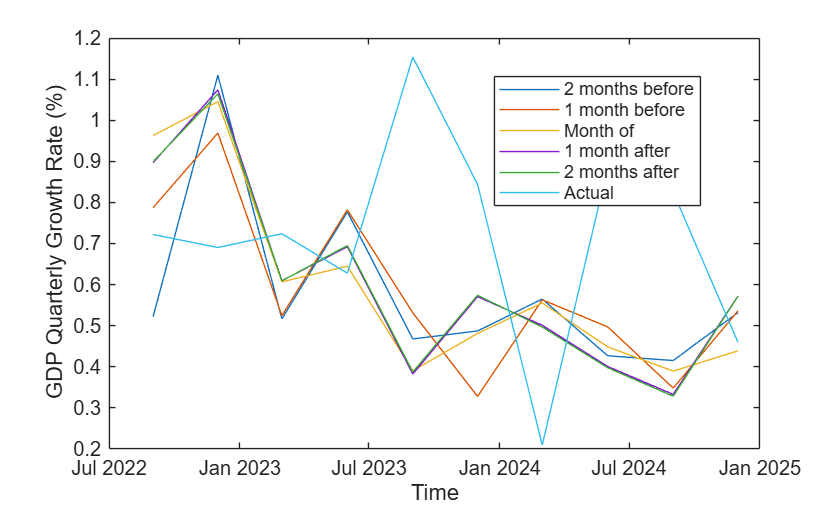
The earliest vintage produces the highest prediction error, and errors decline as more data becomes available, reaching the lowest point at the "month of" vintage. The later vintages do not continue to improve prediction. This suggests that the most informative marginal data arrives in the months leading up to and including the quarter-end, while additional data released afterward adds little predictive value and can introduce minor noise through distributional shift between the training and prediction periods.
Plot the forecast interval for the forecasts at 2-month before target quarter.
idx = DataTbl.Date >= testDateRange(1) - calmonths(15) & DataTbl.Date <=testDateRange(2);
plotData = DataTbl.Variables;
plotData = plotData(idx,end);
times = DataTbl.Date(idx);
idx = ~ismissing(plotData);
plotData = rmmissing(plotData);
times = times(idx);
custom_fanplot(times,plotData*100,Results.Time(1:5:end), ...
    Results.Pred(1:5:end)*100,rmse(Results.Pred(1:5:end)*100,Results.Actual(1:5:end)*100))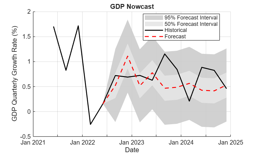
Local Functions
You can call the functions in this section only in this script.
localFetch: Fetch data on variablesinFieldfrom the FRED server using connectionf, and return the data in a timetable.custom_fanplot: Graph ad hoc, custom fan plot.
function outData = localFetch(f,inField)
% localFetch Fetch data from FRED server
% Inputs:
%   f       : FRED connection object
%   inField : String vector of series names
%
% Outputs:
%   outData : Timetable of fetched data
%
    outData = series(f,inField,"observations");
    outData = timetable(outData.observations{1}.date,outData.observations{1}.value,VariableNames=inField);
end

function custom_fanplot(histDates,histData,predDates,predData,rmse_val)
    % Z-scores for 95% intervals
    z_scores = [0.674, 1.96];
    colors = [0.9 0.9 0.9; 0.8 0.8 0.8; 0.7 0.7 0.7];
    interval_labels = ["50% Forecast Interval" "95% Forecast Interval"];

    figure
    hold on

    % Ensure column vectors
    predDates = predDates(:);
    predData = predData(:);
    histDates = histDates(:);
    histData = histData(:);

    % Connect last historical point before predictions
    ind = find(histDates < predDates(1));
    connectedDates = [histDates(ind(end)); predDates];
    connectedData = [histData(ind(end)); predData];

    % Plot the fan bands (largest to smallest)
    for i = numel(z_scores):-1:1
        margin = z_scores(i)*rmse_val(:);

        % Create upper and lower bounds
        upper = [connectedData(1); connectedData(2:end) + margin];
        lower = [connectedData(1); connectedData(2:end) - margin];

        % Create filled polygon with proper label
        fill([connectedDates; flipud(connectedDates)], ...
            [upper; flipud(lower)], ...
            colors(i,:),EdgeColor="none",FaceAlpha=0.9, ...
            DisplayName=interval_labels(i));
    end

    % Plot historical data
    plot(histDates,histData,"k-",LineWidth=1.5,DisplayName="Historical");

    % Plot forecast line (connected to last historical point)
    plot(connectedDates,connectedData,"r--",LineWidth=1.5,DisplayName="Forecast");
    hold off
    grid on
    xlabel("Date")
    ylabel("GDP Quarterly Growth Rate (%)")
    title("GDP Nowcast")
    legend(Location="best")
end
References
See Also
Objects
sequenceInputLayer(Deep Learning Toolbox) |trainingOptions(Deep Learning Toolbox)

