Share Results of Econometric Modeler App Session

This example shows how to share the results of an Econometric Modeler app session by:

Exporting time series and model variables to the MATLAB^® Workspace
Generating MATLAB plain text and live functions to use outside the app
Generating a report of your activities on time series and estimated models

During the session, the example transforms and plots data, runs statistical tests, and estimates a multiplicative seasonal ARIMA model. The data set Data_Airline.mat contains monthly counts of airline passengers.

Import Data into Econometric Modeler

At the command line, load the Data_Airline.mat data set.

load Data_Airline

At the command line, open the Econometric Modeler app.

econometricModeler

Alternatively, open the app from the apps gallery (see Econometric Modeler).

Import DataTimeTable into the app:

On the Econometric Modeler tab, in the Import section, click the Import button .
In the Import Data dialog box, in the Import? column, select the check box for the DataTimeTable variable.
Click Import.

The variable PSSG appears in the Time Series pane, its value appears in the Preview pane, and its time series plot appears in the Time Series Plot(PSSG) figure window.

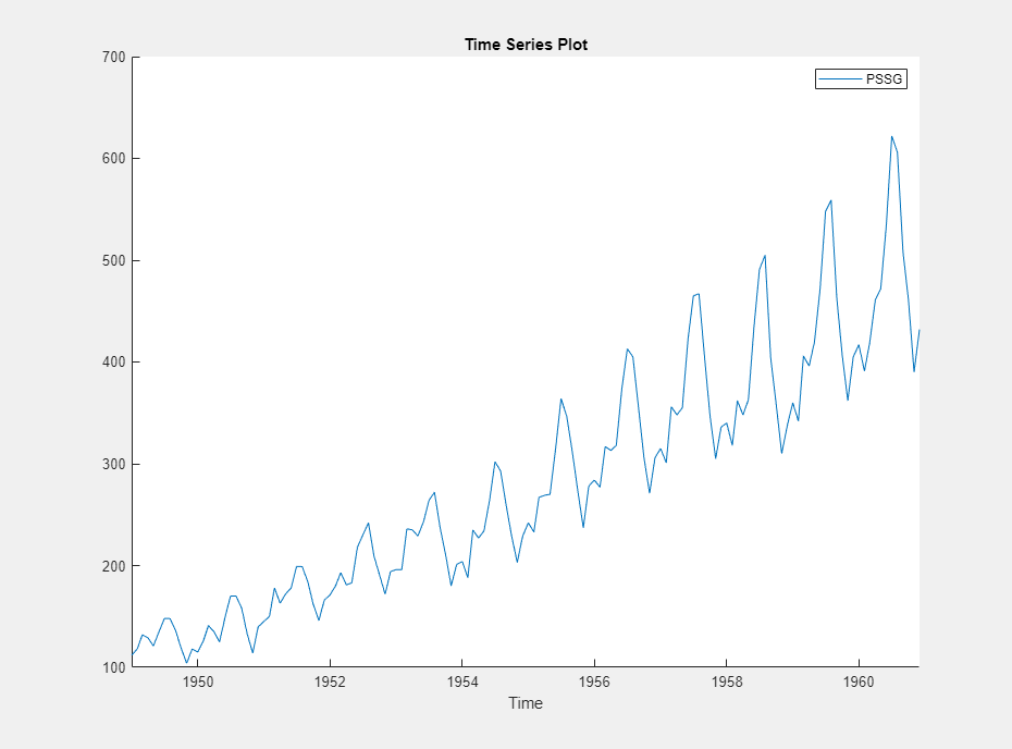
The series exhibits a seasonal trend, serial correlation, and possible exponential growth. For an interactive analysis of serial correlation, see Detect Serial Correlation Using Econometric Modeler App.

Stabilize Series

Address the exponential trend by applying the log transform to PSSG.

In the Time Series pane, select PSSG.
On the Econometric Modeler tab, in the Transforms section, click Log.

The transformed variable PSSGLog appears in the Time Series pane, and its time series plot appears in the Time Series Plot(PSSGLog) figure window.

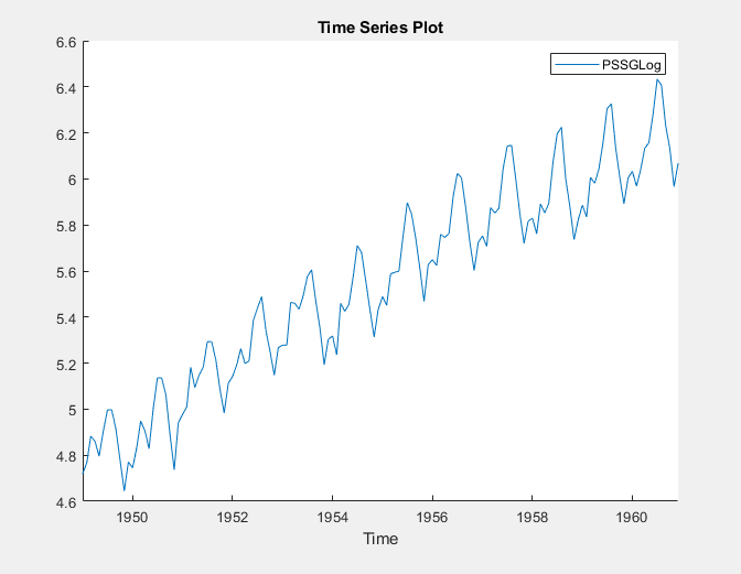
The exponential growth appears to be removed from the series.

Address the seasonal trend by applying the 12th order seasonal difference. With PSSGLog selected in the Time Series pane, on the Econometric Modeler tab, in the Transforms section, set Seasonal to 12. Then, click Seasonal.

The transformed variable PSSGLogSeasonalDiff appears in the Time Series pane, and its time series plot appears in the Time Series Plot(PSSGLogSeasonalDiff) figure window.

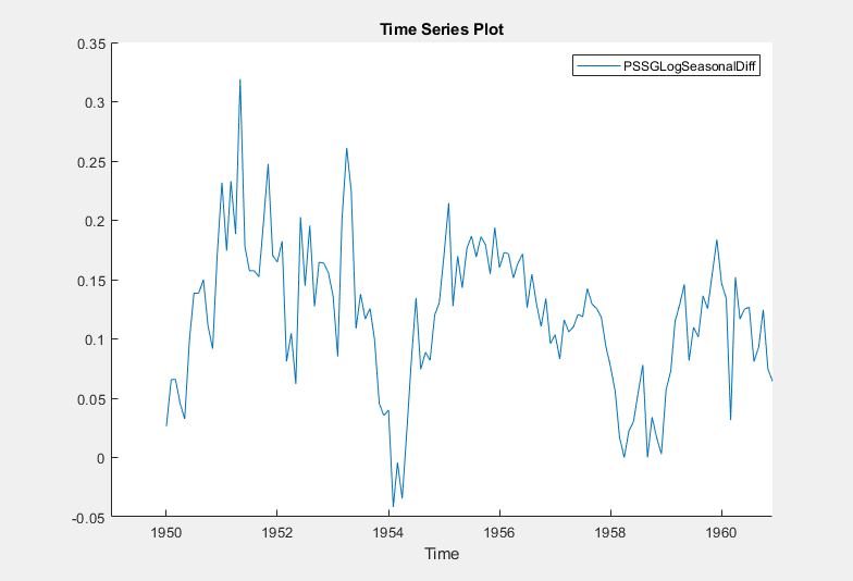
The transformed series appears to have a unit root.

Test the null hypothesis that PSSGLogSeasonalDiff has a unit root by using the Augmented Dickey-Fuller test. Specify that the alternative is an AR(0) model, then test again specifying an AR(1) model. Adjust the significance level to 0.025 to maintain a total significance level of 0.05.

With PSSGLogSeasonalDiff selected in the Time Series pane, on the Econometric Modeler tab, in the Tests section, click New Test > Augmented Dickey-Fuller Test.
On the ADF tab, in the Parameters section, set Significance Level to 0.025.
In the Tests section, click Run Test.
In the Parameters section, set Number of Lags to 1.
In the Tests section, click Run Test.

The test results appear in the Results table of the ADF(PSSGLogSeasonalDiff) document.

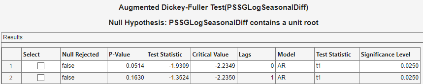
Both tests fail to reject the null hypothesis that the series is a unit root process.

Address the unit root by applying the first difference to PSSGLogSeasonalDiff. With PSSGLogSeasonalDiff selected in the Time Series pane, click the Econometric Modeler tab. Then, in the Transforms section, click Difference.

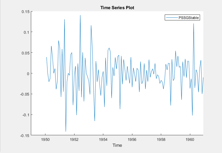
The transformed variable PSSGLogSeasonalDiffDiff appears in the Time Series pane, and its time series plot appears in the Time Series Plot(PSSGLogSeasonalDiffDiff) figure window.

In the Time Series pane, rename the PSSGLogSeasonalDiffDiff variable by clicking it twice to select its name and PSSGStable.

The app updates the names of all documents associated with the transformed series.

Identify Model for Series

Determine the lag structure for a conditional mean model of the data by plotting the sample autocorrelation function (ACF) and partial autocorrelation function (PACF).

With PSSGStable selected in the Time Series pane, click the Plots tab, then click ACF.
Show the first 50 lags of the ACF. On the ACF tab, set Number of Lags to 50.
Click the Plots tab, then click PACF.
Show the first 50 lags of the PACF. On the PACF tab, set Number of Lags to 50.
Drag the ACF(PSSGStable) figure window above the PACF(PSSGStable) figure window.

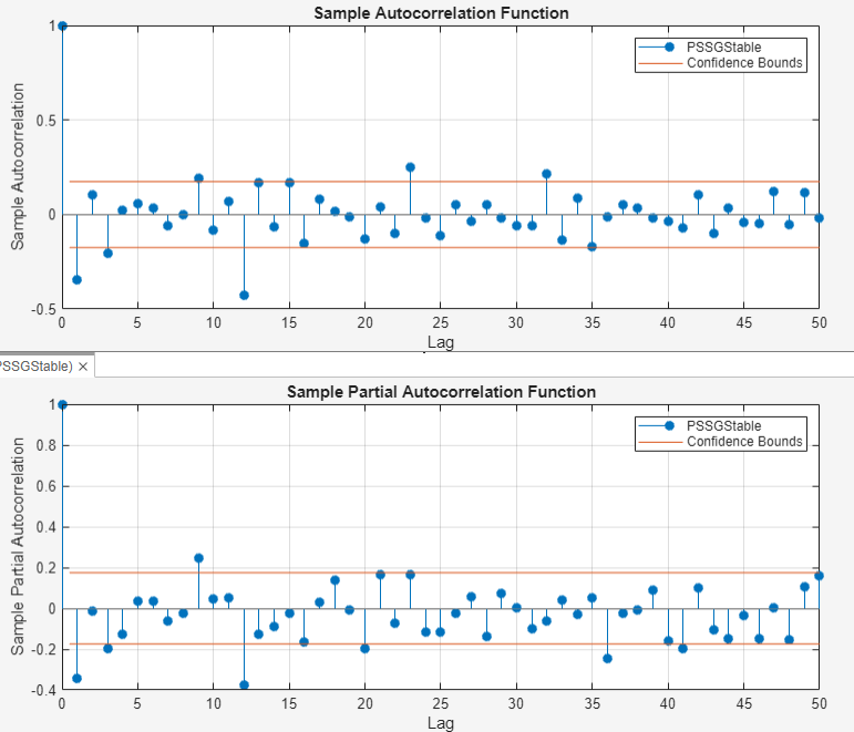
According to [1], the autocorrelations in the ACF and PACF suggest that the following SARIMA(0,1,1)×(0,1,1)₁₂ model is appropriate for PSSGLog.

$(1 - L) (1 - L^{12}) y_{t} = (1 + θ_{1} L) (1 + Θ_{12} L^{12}) ε_{t} .$

Close all figure windows.

Specify and Estimate SARIMA Model

Specify the SARIMA(0,1,1)×(0,1,1)₁₂ model.

In the Time Series pane, select the PSSGLog time series.
On the Econometric Modeler tab, in the Models section, click the arrow to display the models gallery.
In the models gallery, in the ARMA/ARIMA Models section, click SARIMA.
In the SARIMA Model Parameters dialog box, on the Lag Order tab:
- Nonseasonal section
  1. Set Degrees of Integration to 1.
  2. Set Moving Average Order to 1.
  3. Clear the Include Constant Term check box.
- Seasonal section
  1. Set Period to 12 to indicate monthly data.
  2. Set Moving Average Order to 1.
  3. Select the Include Seasonal Difference check box.
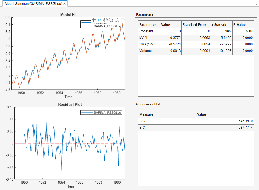
Click Estimate.

The model variable SARIMA_PSSGLog appears in the Models pane, its value appears in the Preview pane, and its estimation summary appears in the Model Summary(SARIMA_PSSGLog) document.

Export Variables to Workspace

Export PSSGLog, PSSGStable, and SARIMA_PSSGLog to the MATLAB Workspace.

On the Econometric Modeler tab, in the Export section, click .
In the Export Variables dialog box, select the Select check boxes for the PSSGLog and PSSGStable time series, and the SARIMA_PSSGLog model (if necessary). The app automatically selects the check boxes for all variables that are highlighted in the Time Series and Models panes.
Click Export.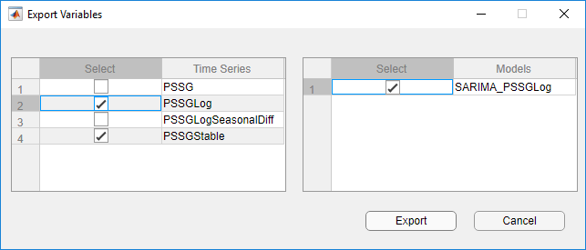

At the command line, list all variables in the workspace.

whos

  Name                  Size            Bytes  Class        Attributes

  Data               144x1              1152  double                 
  DataTable          144x2              3525  table                  
  DataTimeTable      144x1              3311  timetable              
  Description         22x54             2376  char                   
  PSSGLog            144x1              1152  double                 
  PSSGStable         144x1              1152  double                 
  SARIMA_PSSGLog       1x1              7963  arima                  
  dates              144x1              1152  double                 
  series               1x1               162  cell

The contents of Data_Airline.mat, the numeric vectors PSSGLog and PSSGStable, and the estimated arima model object SARIMA_PSSGLog are variables in the workspace.

Forecast the next three years (36 months) of log airline passenger counts using SARIMA_PSSGLog. Specify the PSSGLog as presample data.

numObs = 36;
fPSSG = forecast(SARIMA_PSSGLog,numObs,'Y0',PSSGLog);

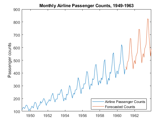
Plot the passenger counts and the forecasts.

fh = DataTimeTable.Time(end) + calmonths(1:numObs);

figure;
plot(DataTimeTable.Time,exp(PSSGLog));
hold on
plot(fh,exp(fPSSG));
legend('Airline Passenger Counts','Forecasted Counts',...
     'Location','best')
title('Monthly Airline Passenger Counts, 1949-1963')
ylabel('Passenger counts')
hold off

Generate Plain Text Function from App Session

Generate a MATLAB function for use outside the app. The function returns the estimated model SARIMA_PSSGLog given DataTimeTable.

In the Models pane of the app, select the SARIMA_PSSGLog model.
On the Econometric Modeler tab, in the Export section, click Export > Generate Function. The MATLAB Editor opens and contains a function named modelTimeSeries. The function accepts DataTimeTable (the variable you imported in this session), transforms data, and returns the estimated SARIMA(0,1,1)×(0,1,1)₁₂ model SARIMA_PSSGLog.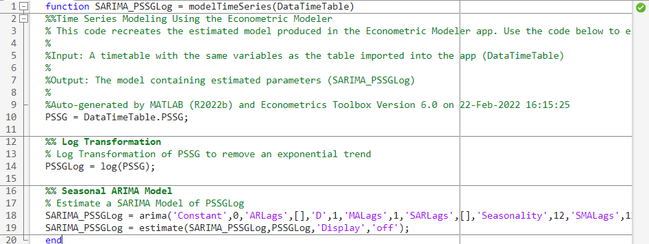
On the Editor tab, click Save > Save.
Save the function to your current folder by clicking Save in the Select File for Save As dialog box.

At the command line, estimate the SARIMA(0,1,1)×(0,1,1)₁₂ model by passing DataTimeTable to modelTimeSeries. Name the model SARIMA_PSSGLog2. Compare the estimated model to SARIMA_PSSGLog.

SARIMA_PSSGLog2 = modelTimeSeries(DataTimeTable);

summarize(SARIMA_PSSGLog)
summarize(SARIMA_PSSGLog2)

   ARIMA(0,1,1) Model Seasonally Integrated with Seasonal MA(12) (Gaussian Distribution)
 
    Effective Sample Size: 144
    Number of Estimated Parameters: 3
    LogLikelihood: 276.198
    AIC: -546.397
    BIC: -537.488
 
                  Value      StandardError    TStatistic      PValue  
                _________    _____________    __________    __________

    Constant            0              0           NaN             NaN
    MA{1}        -0.37716       0.066794       -5.6466      1.6364e-08
    SMA{12}      -0.57238       0.085439       -6.6992      2.0952e-11
    Variance    0.0012634     0.00012395        10.193      2.1406e-24

 
 
 
   ARIMA(0,1,1) Model Seasonally Integrated with Seasonal MA(12) (Gaussian Distribution)
 
    Effective Sample Size: 144
    Number of Estimated Parameters: 3
    LogLikelihood: 276.198
    AIC: -546.397
    BIC: -537.488
 
                  Value      StandardError    TStatistic      PValue  
                _________    _____________    __________    __________

    Constant            0              0           NaN             NaN
    MA{1}        -0.37716       0.066794       -5.6466      1.6364e-08
    SMA{12}      -0.57238       0.085439       -6.6992      2.0952e-11
    Variance    0.0012634     0.00012395        10.193      2.1406e-24

As expected, the models are identical.

Generate Live Function from App Session

Unlike a plain text function, a live function contains formatted text and equations that you can modify by using the Live Editor.

Generate a live function for use outside the app. The function returns the estimated model SARIMA_PSSGLog given DataTimeTable.

In the Models pane of the app, select the SARIMA_PSSGLog model.
On the Econometric Modeler tab, in the Export section, click Export > Generate Live Function. The Live Editor opens and contains a function named modelTimeSeries. The function accepts DataTimeTable (the variable you imported in this session), transforms data, and returns the estimated SARIMA(0,1,1)×(0,1,1)₁₂ model SARIMA_PSSGLog.
To ensure the function does not shadow the M-file function, change the name of the function to modelTimeSeriesMLX.
On the Live Editor tab, in the File section, click Save > Save.
Save the function to your current folder by clicking Save in the Select File for Save As dialog box.

At the command line, estimate the SARIMA(0,1,1)×(0,1,1)₁₂ model by passing DataTimeTable to modelTimeSeriesMLX. Name the model SARIMA_PSSGLog2. Compare the estimated model to SARIMA_PSSGLog.

SARIMA_PSSGLog2 = modelTimeSeriesMLX(DataTimeTable);

summarize(SARIMA_PSSGLog)
summarize(SARIMA_PSSGLog2)

   ARIMA(0,1,1) Model Seasonally Integrated with Seasonal MA(12) (Gaussian Distribution)
 
    Effective Sample Size: 144
    Number of Estimated Parameters: 3
    LogLikelihood: 276.198
    AIC: -546.397
    BIC: -537.488
 
                  Value      StandardError    TStatistic      PValue  
                _________    _____________    __________    __________

    Constant            0              0                        NaN
    MA{1}        -0.37716       0.066794       -5.6466      1.6364e-08
    SMA{12}      -0.57238       0.085439       -6.6992      2.0952e-11
    Variance    0.0012634     0.00012395        10.193      2.1406e-24

 
 
 
   ARIMA(0,1,1) Model Seasonally Integrated with Seasonal MA(12) (Gaussian Distribution)
 
    Effective Sample Size: 144
    Number of Estimated Parameters: 3
    LogLikelihood: 276.198
    AIC: -546.397
    BIC: -537.488
 
                  Value      StandardError    TStatistic      PValue  
                _________    _____________    __________    __________

    Constant            0              0           NaN             NaN
    MA{1}        -0.37716       0.066794       -5.6466      1.6364e-08
    SMA{12}      -0.57238       0.085439       -6.6992      2.0952e-11
    Variance    0.0012634     0.00012395        10.193      2.1406e-24

As expected, the models are identical.

Generate Report

Generate a PDF report of all your actions on the PSSGLog and PSSGStable time series, and the SARIMA_PSSGLog model.

On the Econometric Modeler tab, in the Export section, click Export > Generate Report.
In the Select Variables for Report dialog box, select the Select check boxes for the PSSGLog and PSSGStable time series, and the SARIMA_PSSGLog model (if necessary). The app automatically selects the check boxes for all variables that are highlighted in the Time Series and Models panes.
Click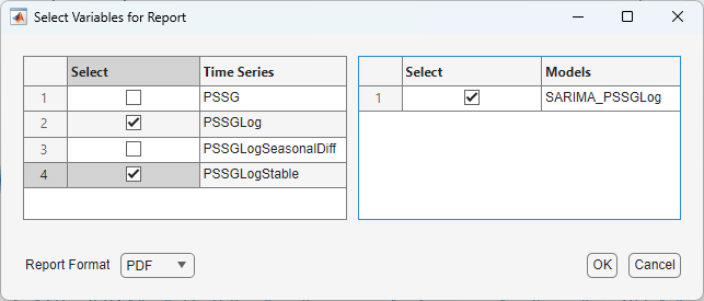 OK.
In the Select File to Write dialog box, navigate to the C:\MyData folder.
In the File name box, type SARIMAReport.
Click Save.

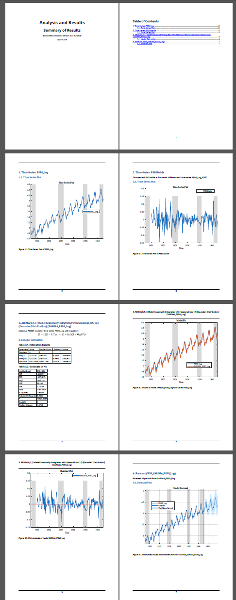
The app publishes the code required to create PSSGLog, PSSGStable, and SARIMA_PSSGLog in the PDF C:\MyData\SARIMAReport.pdf. The report includes:

A title page and table of contents
Plots that include the selected time series
Descriptions of transformations applied to the selected time series
Results of statistical tests conducted on the selected time series
Estimation summaries of the selected models

References

[1] Box, George E. P., Gwilym M. Jenkins, and Gregory C. Reinsel. Time Series Analysis: Forecasting and Control. 3rd ed. Englewood Cliffs, NJ: Prentice Hall, 1994.