Model Data Using Regression and Curve Fitting

This example shows how to execute MATLAB^® data regression and curve fitting in Microsoft^® Excel^® using a worksheet and a VBA macro.

The example organizes and displays the input and output data in a Microsoft Excel worksheet. Spreadsheet Link™ functions copy the data to the MATLAB workspace and execute MATLAB computational and graphic functions. The VBA macro also returns output data to a worksheet.

To work with VBA code in Excel with Spreadsheet Link, you must enable Spreadsheet Link as a reference in the Microsoft Visual Basic^® Editor. For details, see Installation.

Open the ExliSamp.xls file and select the Sheet1 worksheet. For help finding the ExliSamp.xls file, see Installation.

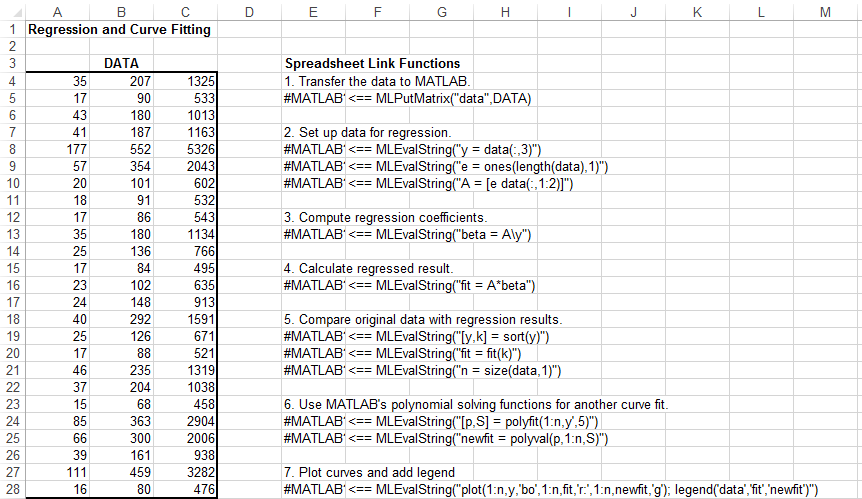
Sheet1 of the spreadsheet contains the named range DATA, which consists of the example data set in worksheet cells A4 through C28.

Model Data in Worksheet

To perform regression and curve fitting, execute the specified Spreadsheet Link functions in worksheet cells.

1. Execute the Spreadsheet Link function that copies the sample data set to the MATLAB workspace by double-clicking the cell E5 and pressing Enter. The data set contains 25 observations of three variables. There is a strong linear dependence among the observations. In fact, they are close to being scalar multiples of each other.

2. Execute the functions in cells E8, E9, and E10. The Spreadsheet Link functions in these cells regress the third column of data on the other two columns, and create:

   • A single vector y containing the third-column data

   • A three-column matrix A, which consists of a column of 1s followed by the rest of the data

3. Execute the function in cell E13. This function calculates the regression coefficients by using the MATLAB back slash (\) operation to solve the overdetermined system of linear equations, A*beta = y.

4. Execute the function in cell E16. MATLAB matrix-vector multiplication produces the regressed result, fit.

5. Execute the functions in cells E19, E20, and E21. These functions:

   1. Compare the original data with fit.

   2. Sort the data in increasing order and apply the same permutation to fit.

   3. Create a scalar for the number of observations.

6. Execute the functions in cells E24 and E25. Fit a polynomial equation to the data for a fifth-degree polynomial. The MATLAB polyfit function automates setting up a system of simultaneous linear equations and solutions for the coefficients. The polyval function then evaluates the resulting polynomial at each data point to check the goodness of the fit newfit.

7. Execute the function in cell E28. The MATLAB plot function graphs the original data (blue circles), the regressed result fit (dashed red line), and the polynomial result (solid green line).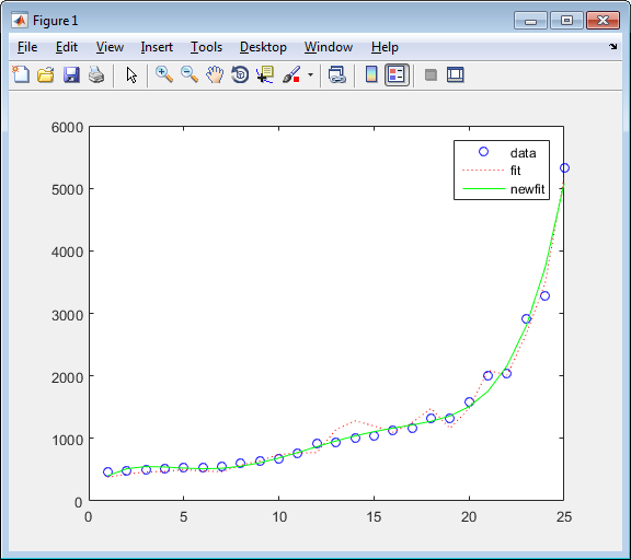

   

   Since the data is closely correlated, but not exactly linearly dependent, the fit curve (dashed line) shows a close, but not exact, fit. The fifth-degree polynomial curve newfit is a more accurate mathematical model for the data.

Model Data Using VBA Macro

To model the data using a VBA macro, execute the Spreadsheet Link functions in a VBA macro.

1. In the ExliSamp.xls file, click the Sheet2 tab. The worksheet for this example appears.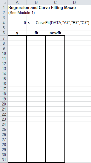

   

   Cell A4 calls the macro CurveFit, which you can examine in the Microsoft Visual Basic environment.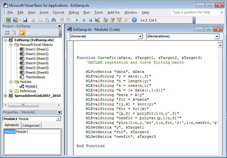

   

   While this module is open, ensure that the Spreadsheet Link add-in is enabled. To enable it, see Add-In Setup. After the add-in is enabled, the Project Explorer lists it under the References folder.

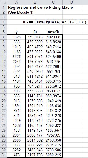
2. Execute the CurveFit macro by double-clicking the cell A4 and pressing Enter. The macro runs the Spreadsheet Link functions. When the macro finishes, the input and output data appears in worksheet cells A7:C31.

   • Column A contains the original data y (sorted).

   • Column B contains the corresponding regressed data fit.

   • Column C contains the polynomial data newfit.