Creating the PortfolioCVaR Object

To create a fully specified CVaR portfolio optimization problem, instantiate the PortfolioCVaR object using PortfolioCVaR. For information on the workflow when using PortfolioCVaR objects, see PortfolioCVaR Object Workflow.

Syntax

Use PortfolioCVaR to create an instance of an object of the PortfolioCVaR class. You can use PortfolioCVaR object in several ways. To set up a portfolio optimization problem in a PortfolioCVaR object, the simplest syntax is:

p = PortfolioCVaR;

This syntax creates a PortfolioCVaR object, p, such that all object properties are empty.

The PortfolioCVaR object also accepts collections of argument name-value pair arguments for properties and their values. The PortfolioCVaR object accepts inputs for public properties with the general syntax:

	p = PortfolioCVaR('property1', value1, 'property2', value2, ... );

If a PortfolioCVaR object already exists, the syntax permits the first (and only the first argument) of PortfolioCVaR to be an existing object with subsequent argument name-value pair arguments for properties to be added or modified. For example, given an existing PortfolioCVaR object in p, the general syntax is:

p = PortfolioCVaR(p, 'property1', value1, 'property2', value2, ... );

Input argument names are not case-sensitive, but must be completely specified. In addition, several properties can be specified with alternative argument names (see Shortcuts for Property Names). The PortfolioCVaR object tries to detect problem dimensions from the inputs and, once set, subsequent inputs can undergo various scalar or matrix expansion operations that simplify the overall process to formulate a problem. In addition, a PortfolioCVaR object is a value object so that, given portfolio p, the following code creates two objects, p and q, that are distinct:

q = PortfolioCVaR(p, ...)

PortfolioCVaR Problem Sufficiency

A CVaR portfolio optimization problem is completely specified with the PortfolioCVaR object if the following three conditions are met:

You must specify a collection of asset returns or prices known as scenarios such that all scenarios are finite asset returns or prices. These scenarios are meant to be samples from the underlying probability distribution of asset returns. This condition can be satisfied by the setScenarios function or with several canned scenario simulation functions.
The set of feasible portfolios must be a nonempty compact set, where a compact set is closed and bounded. You can satisfy this condition using an extensive collection of properties that define different types of constraints to form a set of feasible portfolios. Since such sets must be bounded, either explicit or implicit constraints can be imposed and several tools, such as the estimateBounds function, provide ways to ensure that your problem is properly formulated.
You must specify a probability level to locate the level of tail loss above which the conditional value-at-risk is to be minimized. This condition can be satisfied by the setProbabilityLevel function.
Although the general sufficient conditions for CVaR portfolio optimization go beyond the first three conditions, the PortfolioCVaR object handles all these additional conditions.

PortfolioCVaR Function Examples

If you create a PortfolioCVaR object, p, with no input arguments, you can display it using disp:

p = PortfolioCVaR;
disp(p)

PortfolioCVaR with properties:

                       BuyCost: []
                      SellCost: []
                  RiskFreeRate: []
              ProbabilityLevel: []
                      Turnover: []
                   BuyTurnover: []
                  SellTurnover: []
                  NumScenarios: []
                          Name: []
                     NumAssets: []
                     AssetList: []
                      InitPort: []
                   AInequality: []
                   bInequality: []
                     AEquality: []
                     bEquality: []
                    LowerBound: []
                    UpperBound: []
                   LowerBudget: []
                   UpperBudget: []
                   GroupMatrix: []
                    LowerGroup: []
                    UpperGroup: []
                        GroupA: []
                        GroupB: []
                    LowerRatio: []
                    UpperRatio: []
                  MinNumAssets: []
                  MaxNumAssets: []
    ConditionalBudgetThreshold: []
        ConditionalUpperBudget: []
                     BoundType: []

The approaches listed provide a way to set up a portfolio optimization problem with the PortfolioCVaR object. The custom set functions offer additional ways to set and modify collections of properties in the PortfolioCVaR object.

Using the PortfolioCVaR Function for a Single-Step Setup

You can use the PortfolioCVaR object to directly set up a “standard” portfolio optimization problem. Given scenarios of asset returns in the variable AssetScenarios, this problem is completely specified as follows:

m = [ 0.05; 0.1; 0.12; 0.18 ];
C = [ 0.0064 0.00408 0.00192 0; 
    0.00408 0.0289 0.0204 0.0119;
    0.00192 0.0204 0.0576 0.0336;
    0 0.0119 0.0336 0.1225 ];
m = m/12;
C = C/12;

AssetScenarios = mvnrnd(m, C, 20000);

p = PortfolioCVaR('Scenarios', AssetScenarios, ...
'LowerBound', 0, 'LowerBudget', 1, 'UpperBudget', 1, ...
'ProbabilityLevel', 0.95)

p = 

  PortfolioCVaR with properties:

                       BuyCost: []
                      SellCost: []
                  RiskFreeRate: []
              ProbabilityLevel: 0.9500
                      Turnover: []
                   BuyTurnover: []
                  SellTurnover: []
                  NumScenarios: 20000
                          Name: []
                     NumAssets: 4
                     AssetList: []
                      InitPort: []
                   AInequality: []
                   bInequality: []
                     AEquality: []
                     bEquality: []
                    LowerBound: [4×1 double]
                    UpperBound: []
                   LowerBudget: 1
                   UpperBudget: 1
                   GroupMatrix: []
                    LowerGroup: []
                    UpperGroup: []
                        GroupA: []
                        GroupB: []
                    LowerRatio: []
                    UpperRatio: []
                  MinNumAssets: []
                  MaxNumAssets: []
    ConditionalBudgetThreshold: []
        ConditionalUpperBudget: []
                     BoundType: []

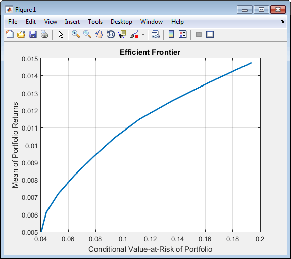
The LowerBound property value undergoes scalar expansion since AssetScenarios provides the dimensions of the problem.

You can use dot notation with the function plotFrontier.

p.plotFrontier

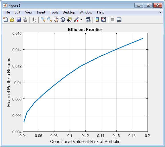
Figure contains a plot for the efficient frontier using a PortfolioCVaR object.

Using the PortfolioCVaR Function with a Sequence of Steps

An alternative way to accomplish the same task of setting up a “standard” CVaR portfolio optimization problem, given AssetScenarios variable is:

m = [ 0.05; 0.1; 0.12; 0.18 ];
C = [ 0.0064 0.00408 0.00192 0;
0.00408 0.0289 0.0204 0.0119;
0.00192 0.0204 0.0576 0.0336;
0 0.0119 0.0336 0.1225 ];

m = m/12;
C = C/12;

AssetScenarios = mvnrnd(m, C, 20000);

p = PortfolioCVaR;
p = setScenarios(p, AssetScenarios);
p = PortfolioCVaR(p, 'LowerBound', 0);
p = PortfolioCVaR(p, 'LowerBudget', 1, 'UpperBudget', 1);
p = setProbabilityLevel(p, 0.95);

plotFrontier(p)

This way works because the calls to the are in this particular order. In this case, the call to initialize AssetScenarios provides the dimensions for the problem. If you were to do this step last, you would have to explicitly dimension the LowerBound property as follows:

m = [ 0.05; 0.1; 0.12; 0.18 ];
C = [ 0.0064 0.00408 0.00192 0;
0.00408 0.0289 0.0204 0.0119;
0.00192 0.0204 0.0576 0.0336;
0 0.0119 0.0336 0.1225 ];

m = m/12;
C = C/12;

AssetScenarios = mvnrnd(m, C, 20000);

p = PortfolioCVaR;
p = PortfolioCVaR(p, 'LowerBound', zeros(size(m)));
p = PortfolioCVaR(p, 'LowerBudget', 1, 'UpperBudget', 1);
p = setProbabilityLevel(p, 0.95);
p = setScenarios(p, AssetScenarios);

Note

If you did not specify the size of LowerBound but, instead, input a scalar argument, the PortfolioCVaR object assumes that you are defining a single-asset problem and produces an error at the call to set asset scenarios with four assets.

Shortcuts for Property Names

The PortfolioCVaR object has shorter argument names that replace longer argument names associated with specific properties of the PortfolioCVaR object. For example, rather than enter 'ProbabilityLevel', the PortfolioCVaR object accepts the case-insensitive name 'plevel' to set the ProbabilityLevel property in a PortfolioCVaR object. Every shorter argument name corresponds with a single property in the PortfolioCVaR object. The one exception is the alternative argument name 'budget', which signifies both the LowerBudget and UpperBudget properties. When 'budget' is used, then the LowerBudget and UpperBudget properties are set to the same value to form an equality budget constraint.

Shortcuts for Property Names

Shortcut Argument Name	Equivalent Argument / Property Name
`ae`	`AEquality`
`ai`	`AInequality`
`assetnames` or `assets`	`AssetList`
`be`	`bEquality`
`bi`	`bInequality`
`budget`	`UpperBudget` and `LowerBudget`
`group`	`GroupMatrix`
`lb`	`LowerBound`
`n` or `num`	`NumAssets`
`level`, `problevel`, or `plevel`	`ProbabilityLevel`
`rfr`	`RiskFreeRate`
`scenario` or `assetscenarios`	`Scenarios`
`ub`	`UpperBound`

For example, this call to the PortfolioCVaR object uses these shortcuts for properties:

m = [ 0.05; 0.1; 0.12; 0.18 ];
C = [ 0.0064 0.00408 0.00192 0;
0.00408 0.0289 0.0204 0.0119;
0.00192 0.0204 0.0576 0.0336;
0 0.0119 0.0336 0.1225 ];

m = m/12;
C = C/12;

AssetScenarios = mvnrnd(m, C, 20000);

p = PortfolioCVaR('scenario', AssetScenarios, 'lb', 0, 'budget', 1, 'plevel', 0.95);
plotFrontier(p)

Direct Setting of Portfolio Object Properties

Although not recommended, you can set properties directly using dot notation, however no error-checking is done on your inputs:

m = [ 0.05; 0.1; 0.12; 0.18 ];
C = [ 0.0064 0.00408 0.00192 0; 
    0.00408 0.0289 0.0204 0.0119;
    0.00192 0.0204 0.0576 0.0336;
    0 0.0119 0.0336 0.1225 ];
m = m/12;
C = C/12;

AssetScenarios = mvnrnd(m, C, 20000);

p = PortfolioCVaR;

p = setScenarios(p, AssetScenarios);
p.ProbabilityLevel = 0.95;

p.LowerBudget = 1;
p.UpperBudget = 1;
p.LowerBound = zeros(size(m));

plotFrontier(p)

Note

Scenarios cannot be assigned directly using dot notation to a PortfolioCVaR object. Scenarios must always be set through either the PortfolioCVaR object, the setScenarios function, or any of the scenario simulation functions.