Multistatic Localization of a Ship Using GPS Illuminations

Since R2025a

This example examines locating and rescuing a ship that gets lost a few kilometers north of Cape Cod during the night. A rescue team stationed at a nearby lighthouse aims at locating the ship. Equipped with a Global Positioning System (GPS) device capable of accessing GPS satellites, they utilize the device to receive GPS signals reflecting off the ship, enabling them to pinpoint its location.

Introduction

Satellite-based localization offers the benefit of broad accessibility to numerous satellites, making it ideal for outdoor rescue operations using multistatic localization techniques. The core principle behind satellite-based multistatic localization is the utilization of Time-Sum-of-Arrival (TSOA) measurements. In this example, the positions of multiple GPS satellites and the GPS device are determined through standard GPS processing. The satellites function as transmit anchors, while the GPS device serves as the receive anchor. Collectively, these anchors establish a multistatic radar system, where each satellite pairs with the GPS device to form a bistatic pair.

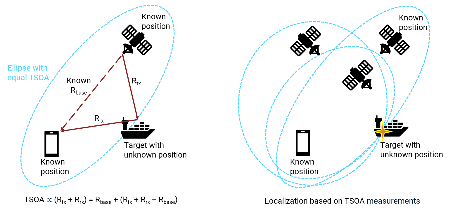
The geometry of a bistatic pair is illustrated in the left figure below. The GPS device receives signals via two paths. The first path (depicted with dashed brown lines) is the direct satellite-to-device path, or baseline, with a known length $$R_{\text{base}}$$. The second path (depicted with solid brown lines) is the satellite-to-target-to-device path, with a combined length of $$R_{\text{tx}}+R_{\text{rx}}$$, where $$R_{\text{tx}}$$ is the satellite-to-target range and $$R_{\text{rx}}$$ is the target-to-device range. This sum, $$R_{\text{tx}}+R_{\text{rx}}$$, defines an ellipsoid of constant range. The left figure shows the ellipsoid when the target, transmitter, and sensor are coplanar. The target is located on the surface of this constant-range ellipsoid, with the satellite and device locations as its foci.

The TSOA is proportional to $$R_{\text{tx}}+R_{\text{rx}}$$. Directly obtaining TSOA is challenging because the exact receive time is difficult to ascertain. However, we can calculate $$R_{\text{tx}}+R_{\text{rx}}$$ by determining the bistatic range $$R_{\text{tx}}+R_{\text{rx}}-R_{\text{base}}$$, since $$R_{\text{base}}$$ is known. The bistatic range is proportional to the Time-Difference-of-Arrival (TDOA) between the target path and the direct path. We can estimate the TDOA by analyzing the arrival time difference of the two paths at the GPS device through spectrum analysis.

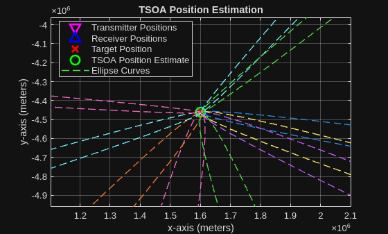
Once TSOA is obtained for each bistatic pair, the GPS device can localize the target. The target's position is at the intersection of the constant-range ellipsoids from different bistatic pairs, as illustrated in the right figure below.

Constant Parameters

Initialize the physical constants required for the simulation.

rng('default')

% RF parameters
fc = 1575.42e6;                                     % Carrier frequency (Hz)
c = physconst('LightSpeed');                        % Speed of propagation (m/s)
lambda = freq2wavelen(fc);                          % Wavelength (m)
bw = 10.23e6;                                       % Bandwidth (Hz)

Satellite Scenario

To create a satellite scenario using the satelliteScenario (Satellite Communications Toolbox) object, define the start time, stop time, and sample time for the scenario. For instance, set the start time to 8:00 AM UTC, which corresponds to 3:00 AM local time at Cape Cod. Use a stop time of 5 minutes to represent the duration of the ship rescue operation.

% Provide the start time
startTime = datetime('2021-06-24 08:00:00',...
    TimeZone="UTC",InputFormat='yyyy-MM-dd HH:mm:ss');

% Initialize satellite scenario
sc = satelliteScenario;
stepTime = 10;                                      % Step time (s)
simDuration = 5;                                    % Simulation duration (min)
sc.StartTime = startTime;
sc.StopTime = sc.StartTime + minutes(simDuration);
sc.SampleTime = stepTime;

Launch the satelliteScenarioViewer (Satellite Communications Toolbox).

viewer = satelliteScenarioViewer(sc);

Use a system effectiveness model (SEM) almanac file to simulate the GPS satellite constellation.

% Set up the GPS satellites based on the almanac file
almFileName = "gpsAlmanac.txt"; 
sat = satellite(sc,almFileName,OrbitPropagator="gps");

Add a GPS device to the satellite scenario by specifying its latitude, longitude, and altitude (LLA).

% Set up the GPS receiver device
rxlat = 42.069322;                                  % Latitude in degrees north
rxlon = -70.245033;                                 % Longitude in degrees east
rxel  = 19;                                         % Elevation in meters
rx = groundStation(sc,rxlat,rxlon,...
    Altitude=rxel,Name="GPS Device"); 

Calculate an access analysis between the GPS device and the satellites. The dashed green lines in the viewer show the line-of-sight access from the GPS device to the satellites.

% Calculate access between GPS satellites and the GPS receiver device
ac = access(sat,rx);
acStats = accessStatus(ac);
satIndices = find(acStats(:,1));
numTx = length(satIndices);
satConnect = sat(satIndices(1:numTx));

Create a geoTrajectory (Satellite Communications Toolbox) System object from a set of LLA waypoints and arrival times typical of a ship. The geoTrajectory System object generates trajectories based on waypoints in geodetic coordinates.

% Set up the ship target
waypoints = [... % Latitude (deg), Longitude (deg), Altitude (meters)
   42.093335, -70.247542, 10;...
   42.101475, -70.219021, 11;...
   42.103852, -70.201065, 12];
timeOfArrival = duration([... % Time (HH:mm:ss)
   "00:00:00";...
   "00:02:40";...
   "00:05:00"]);
trajectory = geoTrajectory(waypoints,seconds(timeOfArrival),...
    AutoPitch=true,AutoBank=true);

Add the ship to the scenario using the platform (Satellite Communications Toolbox) function.

ship = platform(sc,trajectory,Name="Ship");

State Parameters and Platform Configuration

Simulating the entire signal processing flow for the duration of the rescue operation can be time-consuming. Instead, you can simulate specific moments by adjusting the current time index. This allows you to analyze specific events without processing the entire duration.

% Time when the target is estimated
currentTimeIdx = 1;
timeIn = startTime + timeOfArrival(currentTimeIdx);

To set up the signal processing environment, use the states function to obtain the positions and velocities of the satellites and the ship target at the specified time. These are provided in Earth-centered, Earth-fixed (ECEF) coordinates. Use these positions and velocities to configure the phased.Platform (Phased Array System Toolbox) System object for signal propagation.

% Satellite positions
[satpos,satvel] = states(satConnect,timeIn,CoordinateFrame="ecef");
txpos = permute(satpos(:,1,:),[1 3 2]);
txvel = permute(satvel(:,1,:),[1 3 2]);

% Satellite transmitter platform
txplatform = phased.Platform(InitialPosition=txpos,Velocity=txvel); 

% Ship target position
[tgtpos,tgtvel] = states(ship,timeIn,CoordinateFrame="ecef");

% Target platform
tgtplatform = phased.Platform(InitialPosition=tgtpos,Velocity=tgtvel); 

Obtain GPS device position and velocity in ECEF coordinate and use them to configure GPS receiver device platform.

% GPS device position
rxpos = helperLLA2ECEF([rxlat,rxlon,rxel])';
rxvel = zeros(3,1);

% GPS receiver platform
rxplatform = phased.Platform(InitialPosition=rxpos,Velocity=rxvel);

Calculate the ground truth of:

1. Direct-path propagation duration between satellites and the GPS device. The duration is proportional to baseline distance $$R_{\text{base}}$$, and is known at the GPS device following traditional GPS processing.

2. Direct-path Doppler between satellites and the GPS device. The Doppler can be very large and needs to be coarsely estimated at the GPS device before fine-grained range and Doppler estimation.

3. Target-path Time-Sum-of-Arrival (TSOA). The TSOA is proportional to range sum $$R_{\text{tx}}+R_{\text{rx}}$$ of that target-path.

4. Target-path bistatic Doppler.

5. Time-Difference-of-Arrival (TDOA) between target path and direct path.

6. Frequency-Difference-of-Arrival (FDOA) between target path and direct path.

[toadirect,dopdirect,tsoatgt,tdoatgt,fdoatgt] ...
    = helperGroundTruth(c,lambda,tgtpos,tgtvel,txpos,rxpos,txvel,rxvel);

Transceiver Configuration

Create transceiver components for transmitting and receiving signals.

% Tx and Rx parameters
Pt = 44.8;                                          % Peak power (W) 
Gtx = 30;                                           % Tx antenna gain (dB)
Grx = 40;                                           % Rx antenna gain (dB) 
NF = 2.9;                                           % Noise figure (dB) 
fs = bw;                                            % Sample rate (Hz)

% Transceiver components
antenna = phased.IsotropicAntennaElement;
transmitter = phased.Transmitter(Gain=Gtx,PeakPower=Pt);
radiator = phased.Radiator(Sensor=antenna,OperatingFrequency=fc);
collector = phased.Collector(Sensor=antenna,OperatingFrequency=fc);
receiver = phased.Receiver(AddInputNoise=true,Gain=Grx, ...
         NoiseFigure=NF,SampleRate=fs,SeedSource='Property',Seed=0);

GPS Waveform Generation

Obtain navigation configurations and PRN IDs of GPS satellites.

% Generate navigation configuration object
ltncy = latency(sat,rx);
indices = find(~isnan(ltncy(:,1))).';
navcfg = HelperGPSAlmanac2Config(almFileName,...
    "LNAV",indices,startTime);

% Pseudo-random noise (PRN) IDs
availablePRNIDs = [navcfg(:).PRNID];
disp("Available satellites - " + num2str(availablePRNIDs))

Available satellites - 2   4   5   6   9  12  17  19  23  25  29

This figure displays the GPS satellite constellation along with their PRN IDs. The green dotted lines represent the connections between the receiver and the GPS satellites.

Use the gpsWaveformGenerator System object to configure GPS waveforms with the coarse acquisition code (C/A-code) and precision code (P-code). The P-code is assigned to the in-phase (I) branch, while the C/A-code is assigned to the quadrature-phase (Q) branch of the baseband waveform.

% Initialize the GPS waveform generation object
gpswaveobj = gpsWaveformGenerator(SignalType="legacy", ...
    PRNID=availablePRNIDs, ...
    EnablePCode = true,...
    SampleRate=fs, ...
    HasDataWithCACode=true,...
    HasDataWithPCode=true);

A GPS code block lasts 1 millisecond. In multistatic radar signal processing, the GPS device treats each code block as a radar pulse. For Doppler processing, it utilizes multiple pulses.

tPulse = 1e-3;                                      % GPS code block duration (s)
psf = 1/tPulse;                                     % Pulse sending frequency (1/s)
numSamples = fs*tPulse;                             % Number of fast-time samples per pulse
numPulses = 160;                                    % Number slow-time pulses

Generate the navigation data to transmit for all the visible satellites over multiple pulses.

numPulsePerBit = 20;                                % Number of GPS code blocks per bit
numBits = ceil(numPulses/numPulsePerBit);           % Number of transmitted bits

% Navigation data
navdata = randi([0,1],numBits,numTx);        

% GPS waveform with navigation data
waveform_w_data = gpswaveobj(navdata);

Radar Data Cube

Define the bistatic channel as free-space propagation paths. In this example, two classes of channels are modeled:

1. Direct-Path Channel: This channel represents the direct path from a satellite transmitter to the GPS device.

2. Target-Path Channel: This channel includes the path from a satellite transmitter to the ship target and subsequently from the target to the GPS device.

% Configure bistatic channel
[directChannel,tgtChannel] = helperChannel(c,fc,fs);

Due to the high noise floor of the GPS device, caused by Code Division Multiple Access (CDMA) spectrum sharing among multiple GPS satellites, only strong targets are typically observable. In this scenario, we consider a large ship with a high radar cross-section (RCS). You can reduce the RCS to observe its impact on target detection.

% Configure target RCS
tgtrcs = 5e6;                                       % Target RCS (m^2)

The satellite-to-receiver propagation delay is significant. To avoid storing signals over an extended delay during simulation, we use a pseudo path length as the direct-path length. The pseudo path length is specified by the pathOffset variable set to a small value. When pathOffset is 0, the pseudo path length is 0, resulting in a direct-path delay of 0 after ideal signal processing. If the pseudo path length is greater than 0, it represents the synchronization offset between the satellite and the GPS device. Typically, the pathOffset value does not affect the TSOA estimation results, as synchronization errors are eliminated during the TDOA estimation between the target path and the direct path. This delay approximation does not impact path loss calculations, as path loss is determined based on the true signal propagation path.

% Path offset
pathOffset = 0;

Initialize the radar data cube at the GPS device.

% Initialize transmit time
txTime = 0;

% Initialize radr data cube at the GPS device
X = complex(zeros(numSamples,numPulses));

Propagate the GPS waveform through channel using phased transceiver components.

for m = 1:numPulses
    % Update separate transmitter, receiver and target positions
    [tx_pos,tx_vel] = txplatform(tPulse);
    [rx_pos,rx_vel] = rxplatform(tPulse);
    [tgt_pos,tgt_vel] = tgtplatform(tPulse);

    % Transmit waveform
    wave = waveform_w_data((m-1)*numSamples+1:m*numSamples,:);

    for idxTx = 1:numTx
        % Waveform signal
        sig = wave(:,idxTx);

        % Transmitted signal
        txsig = transmitter(sig);

        % Tx-Rx direct path
        ipath = helperGenerateIntPath(tx_pos(:,idxTx),rx_pos, ...
            tx_vel(:,idxTx),rx_vel,lambda);         % True path
        ipath_pseudo = ipath;                       % Pseudo path
        ipath_pseudo.PathLength = pathOffset;

        % Tx-target-Rx path
        tpath = helperGenerateTgtPath(tx_pos(:,idxTx),rx_pos,...
            tx_vel(:,idxTx),rx_vel,tgt_pos,tgt_vel,...
            tgtrcs,lambda);                         % True path
        tpath_pseudo = tpath;                       % Pseudo path
        tpath_pseudo.PathLength = tpath.PathLength - ...
            ipath.PathLength + pathOffset;

        % Radiate signal 
        radsig_tgt = radiator(txsig,...
            tpath_pseudo.AngleOfDeparture);         % Towards the target
        radsig_base = radiator(txsig,...
            ipath_pseudo.AngleOfDeparture);         % Towards the receiver

        % Propagate the signal through Tx-to-target-to-Rx path
        rxsig_tgt = tgtChannel(radsig_tgt,tpath_pseudo,txTime);
        rxsigthis_tgt = rxsig_tgt(:,end);

        % Propagate the signal through Tx-Rx direct path
        rxsig_base = directChannel(radsig_base,ipath_pseudo,txTime);
        rxsigthis_base = rxsig_base(:,end);

        % Collect signal at the receive antenna
        rxsig = collector(rxsigthis_tgt,tpath_pseudo.AngleOfArrival);
        rxsig_ref = collector(rxsigthis_base,ipath_pseudo.AngleOfArrival);

        % Receive signal at the receiver
        X(:,m) = X(:,m) + receiver(rxsig + rxsig_ref);
    end

    % Update transmit time
    txTime = txTime + tPulse;
end

Radar Signal Processing Overview

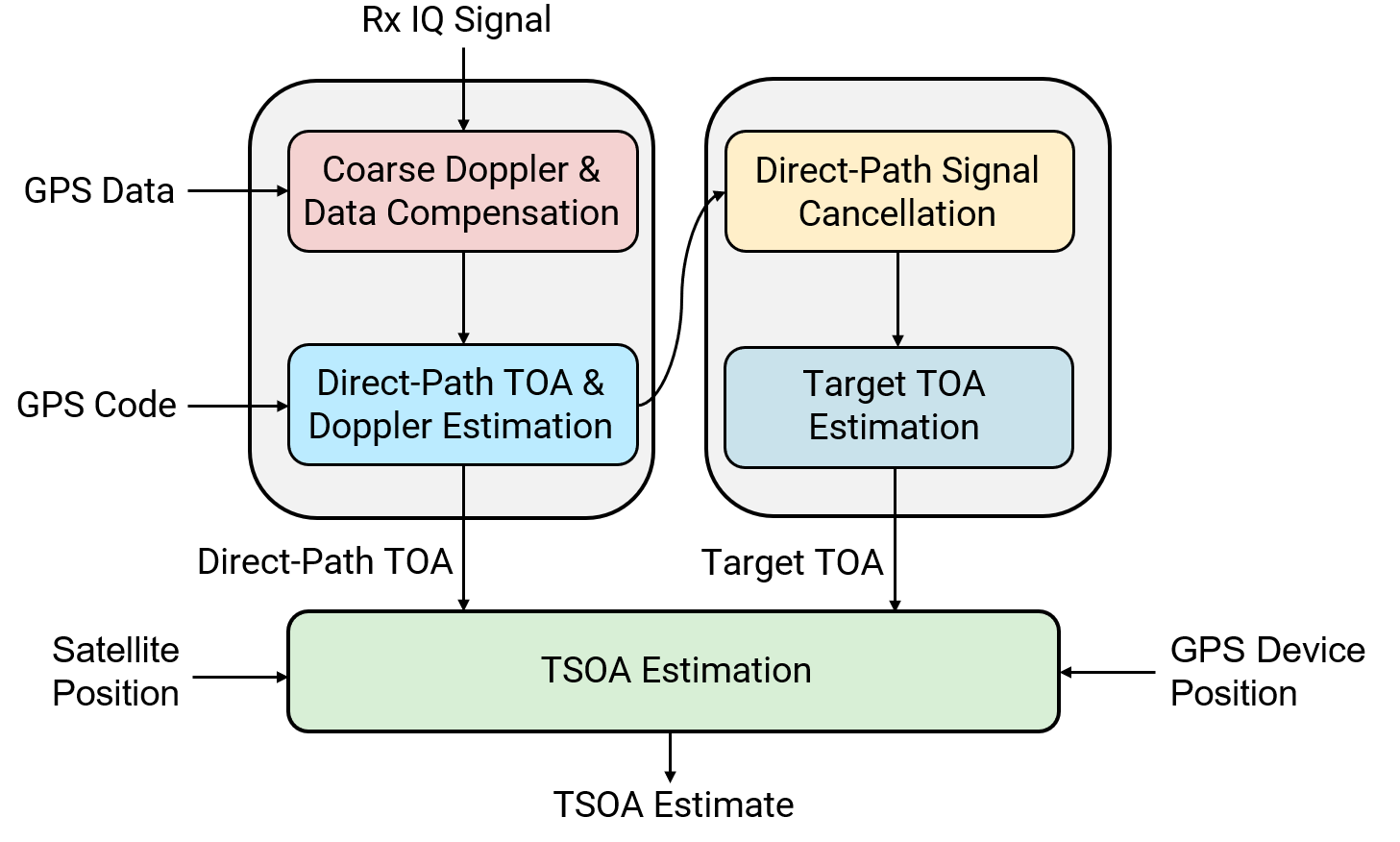
Once the radar data cube (received IQ signal) is obtained, the GPS device aims to estimate the TSOA from each satellite. The high-level signal processing workflow is as follows:

1. Coarse Doppler and Data Compensation: Estimate coarse values of the Doppler offset and apply compensation in the fast-time domain. Due to the rapid movement of satellites, the Doppler shift can be substantial in fast-time domain, resulting in strong range-Doppler coupling. Therefore, it must be compensated in fast-time domain before range processing. Also, compensate the GPS data from the signal. Once the data is removed, the phase between different pulses becomes coherent.

2. Direct-Path TOA and Doppler Estimation: Correlate the compensated signal with the GPS ranging code in fast-time to determine the direct-path Time-of-Arrival (TOA). Also, perform coherent processing of multiple pulses at the detected TOA bin to estimate the direct-path Doppler.

3. Direct-Path Signal Cancellation: Use slow-time domain interference cancellation to significantly reduce direct-path interference.

4. Target TOA Estimation: Estimate the target TOA jointly with the target Doppler to enhance target detectability.

5. TSOA Estimation: Obtain TSOA estimation by combining the TDOA between the direct-path and target signals with the direct-path propagation delay between the satellite and the GPS device.

Direct-Path Pseudo-TOA Estimation

The estimation of the direct-path delay is akin to GPS signal acquisition and involves the following steps:

• Coarse Doppler Compensation: Apply coarse Doppler compensation to the received IQ signal.

• Modulated Data Compensation: Compensate the Doppler-compensated signal for modulated data.

• Correlation with GPS Ranging Code: Correlate the compensated signal with the GPS ranging code to obtain the delay response.

• Noise Floor Estimation: Estimate the noise floor to determine the detection threshold.

• Direct-Path TOA Detection: Detect the TOA on the delay response using the detection threshold.

While standard GPS signal acquisition does not require storing the delay response, in multistatic radar signal processing, the delay response is used for fine-grained direct-path Doppler estimation, which is crucial for direct-path interference cancellation.

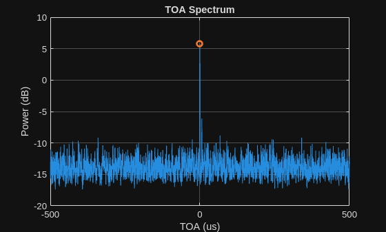
Note that the ideally estimated direct-path TOA equals the pathOffset. This TOA is referred to as the pseudo-TOA, analogous to the pseudo-range concept in standard GPS processing.

% Frquency spacing
freqSpacing = fs/numSamples;

% TOA grid for delay scanning
toaGrid = (-1/2:1/numSamples:1/2-1/numSamples)'/freqSpacing;

% Coarse Doppler compensation matrix
allDopFreq = (-1e4:psf/2:1e4);
dopComp = exp(-1j*2*pi*((0:numSamples-1)/fs).'*allDopFreq);

% Detection threshold factor
dtFactorDirect = 0.9;

% GPS ranging codes for different satellites
refGpsWave = gpsWaveformGenerator(SampleRate=fs,PRNID=availablePRNIDs);
refGpsLongCodes = refGpsWave(zeros(1,length(availablePRNIDs)));
refGpsCodes = refGpsLongCodes(1:numSamples,:)/1j;

psuedoToaEstDirect = zeros(numTx,1);
peakToaDirectIdx = zeros(numTx,1);
toaSpectrumDirect = zeros(numSamples,numTx);
toaResponseDirect = zeros(numSamples,numPulses,numTx);
coarseDopplerIdx = zeros(numTx,1);
for idxTx = 1:numTx
    % Get GPS ranging code
    gpsCode = refGpsCodes(:,idxTx);
    fqyConjCACode = conj(fft(gpsCode,numSamples));

    % Delay-domain response for direct-path
    toaResponse = zeros(numSamples,numPulses);
    
    noiseFloor =  zeros(1,numPulses);
    for m = 1:numPulses
        % Obtain m-th pulse of received signal
        x_m = X(:,m);

        % Compensate Coarse Doppler
        x_m_dop_comp = helperCoarseDopplerCompensation(dopComp,...
            x_m,coarseDopplerIdx,m,idxTx);

        % Compensate modulated data
        x_m_data_comp = helperDataCompensation(x_m_dop_comp,...
            navdata,numPulsePerBit,m,idxTx);
        
        % Obtain direct-path TOA response
        [toaResp,coarseDopplerIdx] = ...
            helperDirectPathTOAResponse(x_m_data_comp,fqyConjCACode,...
            numSamples,coarseDopplerIdx,m,idxTx);
        toaResponse(:,m) = toaResp;

        % Obtain noise floor
        noiseFloor(m) = helperNoiseLevel(x_m_data_comp);
    end
    
    % Detect direct-path TOA
    [toaSpectrum,pkidx] = ...
        helperDirectPathTOADetection(toaResponse,noiseFloor,dtFactorDirect);

    toaResponseDirect(:,:,idxTx) = toaResponse;
    toaSpectrumDirect(:,idxTx) = toaSpectrum;
    psuedoToaEstDirect(idxTx) = toaGrid(pkidx);
    peakToaDirectIdx(idxTx) = pkidx;
end

% Plot TOA spectrum for direct-path psuedo-TOA estimation
idxTxPlot = 1;
helperPlotTOASpectrum(toaSpectrumDirect,toaGrid,peakToaDirectIdx,idxTxPlot)

Direct-Path Pseudo-Doppler Estimation

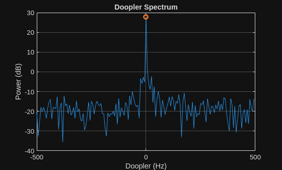
Estimate the direct-path Doppler at the detected delay bin. This estimated Doppler is known as the pseudo-Doppler and will be used for direct-path interference cancellation.

% Doppler grid for Doppler scanning
dopGrid = (-1/2:1/numPulses:1/2-1/numPulses)'*psf;

dopSpectrumDirect = zeros(numPulses,numTx);
psuedoDopEstDirect = zeros(numTx,1);
peakDopDirectIdx = zeros(numTx,1);
for idxTx = 1:numTx
    % Delay response over slow time
    peakToaDirectIdxThis = peakToaDirectIdx(idxTx);
    toaResponsePulse = toaResponseDirect(peakToaDirectIdxThis,:,idxTx);

    % Convert slow-time domain to Doppler domain to obtain Doppler response
    dopResponse = fftshift(fft(toaResponsePulse));

    % Detect direct-path Doppler 
    [dopSpectrum,pkidx] = helperDirectPathDopplerDetection(dopResponse);

    dopSpectrumDirect(:,idxTx) = dopSpectrum;
    psuedoDopEstDirect(idxTx) = dopGrid(pkidx);
    peakDopDirectIdx(idxTx) = pkidx;
end

% Plot Doppler spectrum for direct-path psuedo-Doppler estimation
helperPlotDopplerSpectrum(dopSpectrumDirect,dopGrid,peakDopDirectIdx,idxTxPlot)

Direct-Path Interference Mitigation in Slow-Time Domain

The state-of-the-art method for direct-path interference mitigation is the Enhanced Cancellation Algorithm by Carrier and Doppler Shift (ECA-CD) algorithm. It projects the signal onto the orthogonal subspace of the direct-path interference in the slow-time domain. This interference subspace is calculated using the estimated direct-path pseudo-Doppler.

toaResponseMit = zeros(numSamples,numPulses,numTx);
for idxTx = 1:numTx
    % Delay response
    toaResponseMitThis = toaResponseDirect(:,:,idxTx);

    % Direct-path Doppler frequency
    intDopFreq = psuedoDopEstDirect(idxTx);

    % Mitigate direct-path interference in Doppler-domain 
    toaResponseMit(:,:,idxTx) = helperECACD(toaResponseMitThis,intDopFreq,psf);
end

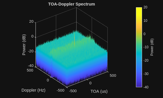
Target-Path Pseudo-TOA-Doppler Estimation

We estimate the target-path pseudo-TOA using the mitigated TOA response. Since the target-path pseudo-TOA is greater than the direct-path pseudo-TOA, only the portion of the mitigated TOA response that occurs after the direct-path pseudo-TOA is used for target TOA estimation. This approach helps avoid false alarms from other parts of the mitigated TOA response. In addition, we jointly process the target signal in TOA-Doppler domain to improve detection probability of the target.

toaDopSpectrumTgt = zeros(numSamples,numPulses,numTx);
pseudoToaTgt = zeros(numTx,1);
pseudoDopTgt = zeros(numTx,1);

for idxTx = 1:numTx
    % Interference-mitigated TOA response
    toaResponseMitThis = toaResponseMit(:,:,idxTx);

    % Obtain target TOA-Doppler response
    toadopResponse = fftshift(fft(toaResponseMitThis,numPulses,2),2);

    % Detect target-path TOA and Doppler
    [toadopSpectrum,maxToaIdx,maxDopIdx] = ...
        helperTargetPathTOADopplerDetection(toadopResponse,peakToaDirectIdx,idxTx);

    toaDopSpectrumTgt(:,:,idxTx) = toadopSpectrum;
    pseudoToaTgt(idxTx) = toaGrid(peakToaDirectIdxThis+maxToaIdx);
    pseudoDopTgt(idxTx) = dopGrid(maxDopIdx(maxToaIdx));
end

% Plot target psuedo-TOA-Doppler spectrum
helperPlotTOADopplerSpectrum(toaDopSpectrumTgt,toaGrid,dopGrid,idxTxPlot)

Following this step, we can determine the TDOA between the target-path and the direct-path by subtracting the direct-path pseudo-TOA from the target-path pseudo-TOA. The path offset specified in pathOffset typically does not affect the TDOA estimate because the common synchronization error in these two paths is canceled out by this subtraction. We can then compare the estimated TDOA with the true TDOA calculated at the beginning of this example.

% Estimate TDOA
tdoatgtest = pseudoToaTgt - psuedoToaEstDirect;

% TDOA estimation error
tdoatgtesterr = tdoatgtest'-tdoatgt;
disp("TDOA Estimate Error (ns) - " + num2str(tdoatgtesterr*1e9))

TDOA Estimate Error (ns) - -3.377657923       19.4992198     -6.252540035      41.75506463      445466.7048     -1.656236177      46.77467529      53.50400294     -30.88228814     -47.96407369      27.49009479

We can also obtain the Frequency-Difference-of-Arrival (FDOA) between the target-path and the direct-path by subtracting the direct-path pseudo-Doppler from the target-path pseudo-Doppler. This estimated FDOA can then be compared with the true FDOA calculated at the beginning of this example.

% Estimate FDOA
fdoatgtest = pseudoDopTgt-psuedoDopEstDirect;

% Doppler estimation error
dopplertgtesterr = fdoatgtest'-fdoatgt;
disp("Doppler Estimate Error (Hz) - " + num2str(dopplertgtesterr))

Doppler Estimate Error (Hz) - 1.0517      2.98578     0.705105     -1.78193      21.0648      1.74473      1.27404     -2.09277      4.54106    -0.709348      2.13353

TSOA Estimation

The TSOA estimation involves the following steps:

1. Obtain TDOA: Calculate the TDOA between the target path and the direct path. This is derived from the bistatic range $$R_{\text{tx}}+R_{\text{rx}}-R_{\text{base}}$$ divided by the propagation speed.

2. Gate False TDOA: Filter out any extremely large TDOA estimates by gating them according to the maximum possible TDOA.

3. Calculate TSOA: Add the known direct-path propagation time to the TDOA to obtain the TSOA. This is equivalent to estimating the range sum $$R_{\text{tx}}+R_{\text{rx}}$$ by adding the bistatic range $$R_{\text{tx}}+R_{\text{rx}}-R_{\text{base}}$$ to the known baseline range $$R_{\text{base}}$$.

% Gate false TDOA
maxrngdiff = 12e3;
maxtdoa = maxrngdiff/c;
tdoatgtest(tdoatgtest>maxtdoa) = nan;

The direct-path propagation time, or baseline range $$R_{\text{base}}$$, is known because we assume that both the satellite positions and the GPS device position are determined using standard GPS processing. Typically, a GPS device requires at least 50 seconds of data to estimate its position as well as the positions of the satellites. The standard procedure for estimating GPS satellite positions is covered in the "GPS Receiver Acquisition and Tracking Using C/A-Code (Satellite Communications Toolbox)" example. In this example, we assume that 50 seconds have already elapsed before commencing this radar signal processing.

% Estimate TSOA
tsoatgtest = tdoatgtest + toadirect';

% TSOA estimation error
tsoatgtesterr = tsoatgtest'-tsoatgt;
disp("TSOA Estimate Error (ns) - " + num2str(tsoatgtesterr*1e9))

TSOA Estimate Error (ns) - -3.377658      19.49922      -6.25254      41.75506           NaN     -1.656236      46.77468        53.504     -30.88229     -47.96407      27.49009

TSOA Position Estimation

For multistatic radar processing, it is necessary to obtain TSOA estimates from at least four satellites to the device, as well as the location of each satellite in the sky at the time of transmission. If the GPS device successfully acquires this information, it can utilize the TSOA position estimation algorithm, implemented in tsoaposest, to estimate the position of the ship target.

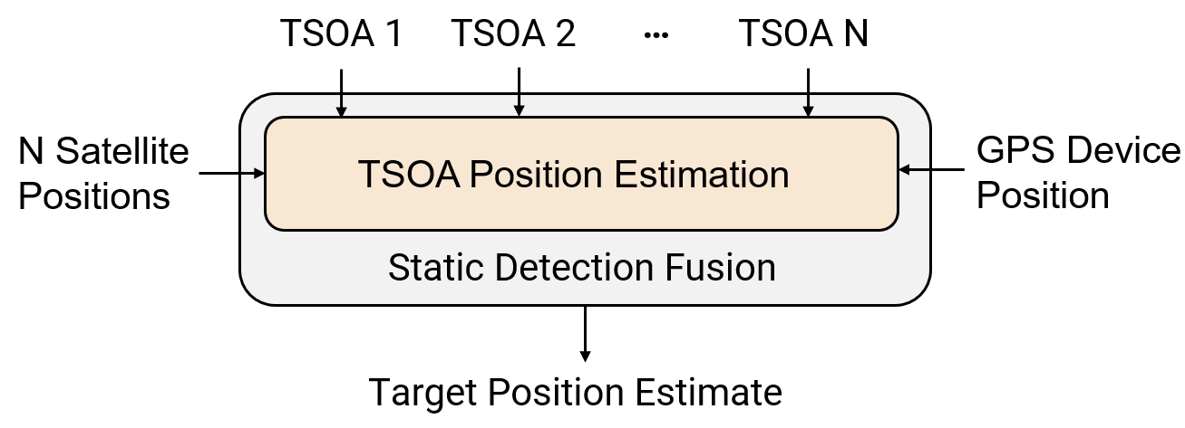
Occasionally, TSOA estimates may include false alarms. To prevent these erroneous estimates from impacting target position estimation, association algorithms can be employed to select valid TSOA estimates. In this example, we can enhance the accuracy of TSOA position estimation by combining tsoaposest with the association algorithm implemented in the staticDetectionFuser System object.

% Approximate TSOA estimation variance
tsoavar = (1/fs)^2*ones(numTx,1);

% Flag to indicate if Sensor Fusion and Tracking Toolbox is licensed
useFusionToolbox = false;

if useFusionToolbox
    % Obtain non-nan TSOA measurements and its corresponding tx position
    nonnanidx = ~isnan(tsoatgtest); %#ok<UNRCH>
    tsoatgtestvalid = tsoatgtest(nonnanidx);
    tsoavarvalid = tsoavar(nonnanidx);
    txposvalid = txpos(:,nonnanidx);

    % Define a static detection fuser
    tsoaFuser = staticDetectionFuser(MaxNumSensors=sum(nonnanidx), ...
        MeasurementFormat='custom', ...
        MeasurementFcn=@helperFusedTSOA, ...
        MeasurementFusionFcn=@helperTSOA2Pos, ...
        FalseAlarmRate=1e-10, ...
        DetectionProbability=0.99, ...
        Volume=1e-2);

    % Detect TSOA
    tsoaDets = helperTSOADetection(tsoatgtestvalid,tsoavarvalid,txposvalid,rxpos);

    % Detect target position
    posDets = tsoaFuser(tsoaDets);

    % Obtain estimated target position
    tgtposest = posDets{1}.Measurement;
else
    % Estimate target position 
    tgtposest = tsoaposest(tsoatgtest,tsoavar,txpos,rxpos);
end

% Position estimation RMSE
posrmse = rmse(tgtposest,tgtpos);
disp("Position Estimation RMSE (m) - " + num2str(posrmse))

Position Estimation RMSE (m) - 6.2192

% Convert ship target position from ECEF to LLA
tgtposestlla = helperECEF2LLA(tgtposest');

View TSOA position estimate on a 2D ECEF plane:

helperPlotTSOAPositions(c,tsoatgtest,tgtposest,txpos,rxpos,tgtpos)

Zoom in to estimation area:

helperZoomInToEstimationArea(tgtposest)

Visualization of Ship Target Estimate

By executing the above simulation across multiple time indices, as specified in currentTimeIdx, we can obtain estimated ship target positions, tgtposestlla, at various waypoints.

% Set up the estimated ship target positions
waypointsest = [... % Latitude (deg), Longitude (deg), Altitude (meters)
   42.093401, -70.247620, 14;...
   42.101478, -70.219038, 12;...
   42.103846, -70.201110, 28];

The accuracy of these ship position estimates over time can be visualized using the Satellite Scenario Viewer.

trajectoryest = geoTrajectory(waypointsest,seconds(timeOfArrival),AutoPitch=true,AutoBank=true);
shipEst = platform(sc,trajectoryest, Name="Ship Estimate");

The Satellite Scenario Viewer display demonstrates that the estimated ship positions are accurate.

Conclusion

This example demonstrates the process of estimating a ship target's position using GPS signals from multiple satellites. Specifically, it demonstrates how to configure a satellite scenario, generate GPS waveforms, propagate waveforms through bistatic channels, perform radar signal processing to obtain TSOA estimates, use TSOA estimates to determine target's position, and visualize the target trajectory on Satellite Scenario Viewer.

Reference

[1] M. Sadeghi, F. Behnia and R. Amiri, "Maritime Target Localization from Bistatic Range Measurements in Space-Based Passive Radar," in IEEE Transactions on Instrumentation and Measurement, vol. 70, pp. 1-8, 2021, Art no. 8502708.

[2] K. Gronowski, P. Samczyński, K. Stasiak and K. Kulpa, "First results of air target detection using single channel passive radar utilizing GPS illumination," 2019 IEEE Radar Conference (RadarConf), Boston, MA, USA, 2019.

[3] C. Schwark and D. Cristallini, "Advanced multipath clutter cancellation in OFDM-based passive radar systems," 2016 IEEE Radar Conference, Philadelphia, PA, USA, 2016, pp. 1-4.

[4] Hugh Griffiths; Christopher Baker, An Introduction to Passive Radar, Second Edition, Artech, 2022.

[5] David A. Vallado, Wayne D. McClain, Fundamentals of Astrodynamics and Applications, Third Edition, Microcosm Press/Springer, 2007.

[6] IS-GPS-200, Rev: M. NAVSTAR GPS Space Segment/Navigation User Interfaces. May 21, 2021; Code Ident: 66RP1.

[7] F. Colone, F. Filippini and D. Pastina, "Passive Radar: Past, Present, and Future Challenges," in IEEE Aerospace and Electronic Systems Magazine, vol. 38, no. 1, pp. 54-69, 1 Jan. 2023.