Predict Chaotic Time Series Using Type-2 FIS
This example shows chaotic time series prediction using a tuned type-2 fuzzy inference system (FIS). This example tunes the FIS using particle swarm optimization, which requires Global Optimization Toolbox software.
Time Series Data
This example simulates time-series data using the following form of the Mackey-Glass (MG) nonlinear delay differential equation.
Simulate the time series for 1200 samples using the following configuration.
Sample time sec
Initial condition
for .
ts = 1;
numSamples = 1200;
tau = 20;
x = zeros(1,numSamples+tau+1);
x(tau+1) = 1.2;
for t = 1+tau:numSamples+tau
    x_dot = 0.2*x(t-tau)/(1+(x(t-tau))^10)-0.1*x(t);
    x(t+1) = x(t) + ts*x_dot;
end
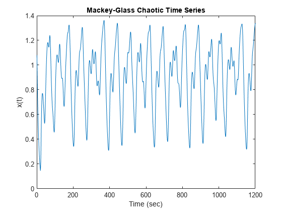
Plot the simulated MG time-series data.
figure(1)
plot(x(tau+2:end))
title("Mackey-Glass Chaotic Time Series")
xlabel("Time (sec)")
ylabel("x(t)")
Generate Training and Validation Data
Time-series prediction uses known time-series values up to time t to predict a future value at time . The standard method for this type of prediction is to create a mapping from D sample data points, sampled every Δ units in time () to a predicted future value . For this example, set and . Hence, for each t, the input and output training data sets are and , respectively. In other words, use four successive known time-series values to predict the next value.
Create 1000 input/output data sets from samples to
D = 4;
inputData = zeros(1000,D);
outputData = zeros(1000,1);
for t = 100+D-1:1100+D-2
    for i = 1:D
        inputData(t-100-D+2,i) = x(t-D+i);
    end
    outputData(t-100-D+2,:) = x(t+1);
end
Use the first 500 data sets as training data (trnX and trnY) and the second 500 sets as validation data (vldX and vldY).
trnX = inputData(1:500,:);
trnY = outputData(1:500,:);
vldX = inputData(501:end,:);
vldY = outputData(501:end,:);
Construct FIS
This example uses a type-2 Sugeno FIS. Since a Sugeno FIS has fewer tunable parameters than a Mamdani FIS, a Sugeno system generally converges faster during optimization.
fisin = sugfistype2;
Add three inputs, each with three default triangular membership functions (MFs). Initially, eliminate the footprint of uncertainty (FOU) for each input MF by setting each lower MF equal to its corresponding upper MF. To do so, set the scale and lag values of each lower MF to 1 and 0, respectively. By eliminating the FOU for all input membership functions, you configure the type-2 FIS to behave like a type-1 FIS.
numInputs = D;
numInputMFs = 3;
range = [min(x) max(x)];
for i = 1:numInputs
    fisin = addInput(fisin,range,NumMFs=numInputMFs);
    for j = 1:numInputMFs
        fisin.Inputs(i).MembershipFunctions(j).LowerScale = 1;
        fisin.Inputs(i).MembershipFunctions(j).LowerLag = 0;
    end
end
For prediction, add an output to the FIS. The output contains default constant membership functions. To provide maximum resolution for the input-output mapping, set the number of output MFs equal to the number of input MF combinations.
numOutputMFs = numInputMFs^numInputs;
fisin = addOutput(fisin,range,NumMFs=numOutputMFs);
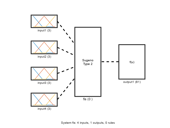
View the FIS structure. Initially, the FIS has zero rules. The rules of the system are found during the tuning process.
plotfis(fisin)
Tune FIS with Training Data
To tune the FIS, you use the following three steps.
Learn the rule base while keeping the input and output MF parameters constant.
Tune the output MF parameters and the upper MF parameters of the inputs while keeping the rule and lower MF parameters constant.
Tune the lower MF parameters of the inputs while keeping the rule, output MF, and upper MF parameters constant.
The first step is less computationally expensive due to the small number of rule parameters, and it quickly converges to a fuzzy rule base during training. After the second step, the system is a trained type-1 FIS. The third step produces a tuned type-2 FIS.
Learn Rules
To learn a rule base, first specify tuning options using a tunefisOptions object.
options = tunefisOptions;
Since the FIS does not contain any pretuned fuzzy rules, use a global optimization method (genetic algorithm or particle swarm) to learn the rules. Global optimization methods perform better in large parameter tuning ranges as compared to local optimization methods (pattern search and simulated annealing). For this example, tune the FIS using particle swarm optimization ("particleswarm").
options.Method = "particleswarm";To learn new rules, set the OptimizationType to "learning".
options.OptimizationType = "learning";Restrict the maximum number of rules to the number of input MF combinations. The number of tuned rules can be less than this limit, since the tuning process removes duplicate rules.
options.NumMaxRules = numInputMFs^numInputs;
If you have Parallel Computing Toolbox™ software, you can improve the speed of the tuning process by setting UseParallel to true. If you do not have Parallel Computing Toolbox software, set UseParallel to false.
options.UseParallel = false;
Set the maximum number of iterations to 10. Increasing the number of iterations can reduce training error. However, the larger number of iterations increases the duration of the tuning process and can overtune the rule parameters to the training data.
options.MethodOptions.MaxIterations = 10;
Since particle swarm optimization uses random search, to obtain reproducible results, initialize the random number generator to its default configuration.
rng("default")Tuning a FIS using the tunefis function takes several minutes. For this example, enable tuning by setting runtunefis to true. To load pretrained results without running tunefis, you can set runtunefis to false.
runtunefis = false;
Tune the FIS using the specified training data and options.
if runtunefis
    fisout1 = tunefis(fisin,[],trnX,trnY,options);
else
    tunedfis = load("tunedfischaotictimeseriestype2.mat");
    fisout1 = tunedfis.fisout1;
end
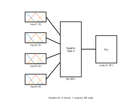
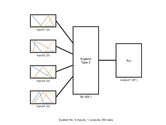
View the structure of the trained FIS, which contains the new learned rules.
plotfis(fisout1)
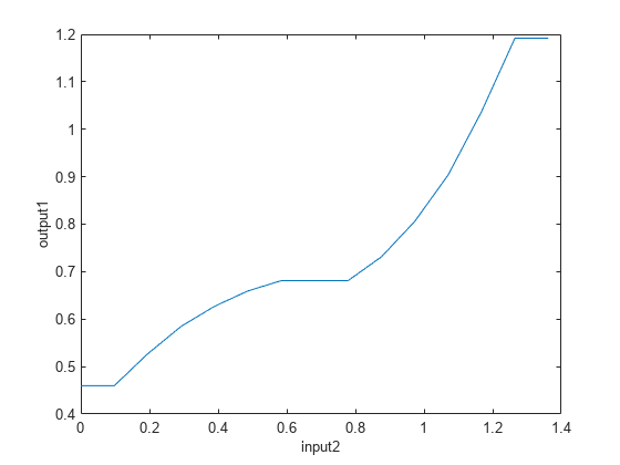
Check the individual input-output relationships tuned by the learned rule base. For example, the following figure shows the relationship between the second input and the output.
gensurf(fisout1,gensurfOptions(InputIndex=2))
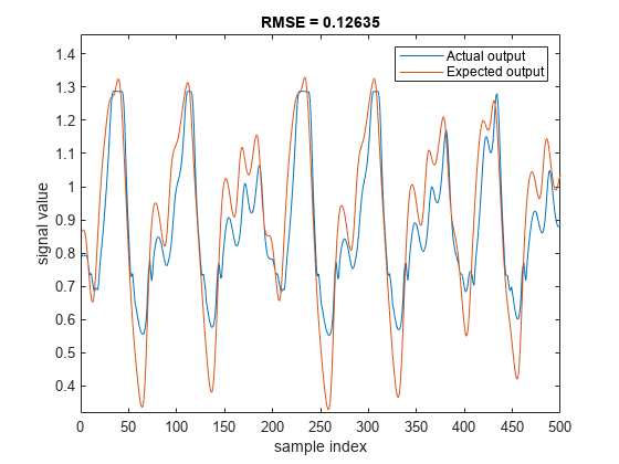
Evaluate the tuned FIS using the input validation data. Plot the actual generated output with the expected validation output, and compute the root mean squared error (RMSE).
plotActualAndExpectedResultsWithRMSE(fisout1,vldX,vldY)
Tune Upper Membership Function Parameters
Tune the upper membership function parameters. A type-2 Sugeno FIS supports only crisp output functions. Therefore, this step tunes input upper MFs and crisp output functions.
Obtain the input and output parameter settings using getTunableSettings. Since the FIS uses triangular input MFs, you can tune the input MFs using asymmetric lag values.
[in,out] = getTunableSettings(fisout1,AsymmetricLag=true);
Disable the tuning of lower MF parameters.
for i = 1:length(in)
    for j = 1:length(in(i).MembershipFunctions)
        in(i).MembershipFunctions(j).LowerScale.Free = false;
        in(i).MembershipFunctions(j).LowerLag.Free = false;
    end
end
To optimize the existing tunable MF parameters while keeping the rule base constant, set OptimizationType to "tuning".
options.OptimizationType = "tuning";Tune the FIS using the specified tuning data and options. To load pretrained results without running tunefis, you can set runtunefis to false.
rng("default")
if runtunefis
    fisout2 = tunefis(fisout1,[in;out],trnX,trnY,options);
else
    tunedfis = load("tunedfischaotictimeseriestype2.mat");
    fisout2 = tunedfis.fisout2;
end
View the structure of the trained FIS, which now contains tuned upper MF parameters.
plotfis(fisout2)
Evaluate the tuned FIS using the validation data, compute the RMSE, and plot the actual generated output with the expected validation output.
plotActualAndExpectedResultsWithRMSE(fisout2,vldX,vldY)
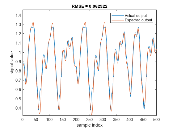
Tuning the upper MF parameters improves the performance of the FIS. This result is equivalent to tuning a type-1 FIS.
Tune Lower Membership Function Parameters
Tune only the input lower MF parameters. To do so, set the lower scale and lag values tunable, and disable tuning of the upper MF parameters.
for i = 1:length(in)
    for j = 1:length(in(i).MembershipFunctions)
        in(i).MembershipFunctions(j).UpperParameters.Free = false;
        in(i).MembershipFunctions(j).LowerScale.Free = true;
        in(i).MembershipFunctions(j).LowerLag.Free = true;
    end
end
Tune the FIS using the specified tuning data and options. To load pretrained results without running tunefis, you can set runtunefis to false.
rng("default")
if runtunefis
    fisout3 = tunefis(fisout2,in,trnX,trnY,options);
else
    tunedfis = load("tunedfischaotictimeseriestype2.mat");
    fisout3 = tunedfis.fisout3;
end
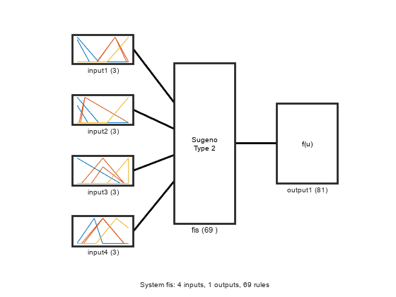
View structure of the trained FIS, which now contains tuned lower MF parameters.
plotfis(fisout3)
Evaluate the tuned FIS using the validation data, compute the RMSE, and plot the actual generated output with the expected validation output.
plotActualAndExpectedResultsWithRMSE(fisout3,vldX,vldY)

Tuning both the upper and lower MF values improves the FIS performance. The RMSE improves when the trained FIS includes both tuned upper and lower parameter values.
Conclusion
Type-2 MFs provides additional tunable parameters as compared to type-1 MFs. Therefore, with adequate training data, a tuned type-2 FIS can fit the training data better than a tuned type-1 FIS.
Overall, you can produce different tuning results by modifying any of the following FIS properties or tuning options:
Number of inputs
Number of MFs
Type of MFs
Optimization method
Number of tuning iterations
Local Functions
function [rmse,actY] = calculateRMSE(fis,x,y)

% Specify options for FIS evaluation.
evalOptions = evalfisOptions( ...
    EmptyOutputFuzzySetMessage="none", ...
    NoRuleFiredMessage="none", ...
    OutOfRangeInputValueMessage="none");

% Evaluate FIS.
actY = evalfis(fis,x,evalOptions);

% Calculate RMSE.
del = actY - y;
rmse = sqrt(mean(del.^2));

end

function plotActualAndExpectedResultsWithRMSE(fis,vldX,vldY)
[rmse,actY] = calculateRMSE(fis,vldX,vldY);

figure
plot([actY vldY])
axis([0 length(vldY) min(vldY)-0.01 max(vldY)+0.13])
xlabel("sample index")
ylabel("signal value")
title("RMSE = " + num2str(rmse))
legend(["Actual output" "Expected output"],Location="northeast")
end