Cette page a été traduite par traduction automatique. Cliquez ici pour voir la dernière version en anglais.

Trouver des minima globaux ou locaux multiples

Cet exemple illustre comment GlobalSearch trouve efficacement un minimum global et comment MultiStart trouve beaucoup plus de minima locaux.

La fonction objectif de cet exemple comporte de nombreux minimums locaux et un minimum global unique. En coordonnées polaires, la fonction est

$f (r, t) = g (r) h (t)$

où

$\begin{array}{l} g (r) = (\sin (r) - \frac{\sin (2 r)}{2} + \frac{\sin (3 r)}{3} - \frac{\sin (4 r)}{4} + 4) \frac{r^{2}}{r + 1} \\ h (t) = 2 + \cos (t) + \frac{\cos (2 t - \frac{1}{2})}{2} . \end{array}$

Tracez les fonctions $g$ et $h$ et créez un graphique de surface de la fonction $f$ .

figure
subplot(1,2,1);
fplot(@(r)(sin(r) - sin(2*r)/2 + sin(3*r)/3 - sin(4*r)/4 + 4) .* r.^2./(r+1), [0 20])
title(''); ylabel('g'); xlabel('r');
subplot(1,2,2);
fplot(@(t)2 + cos(t) + cos(2*t-1/2)/2, [0 2*pi])
title(''); ylabel('h'); xlabel('t');

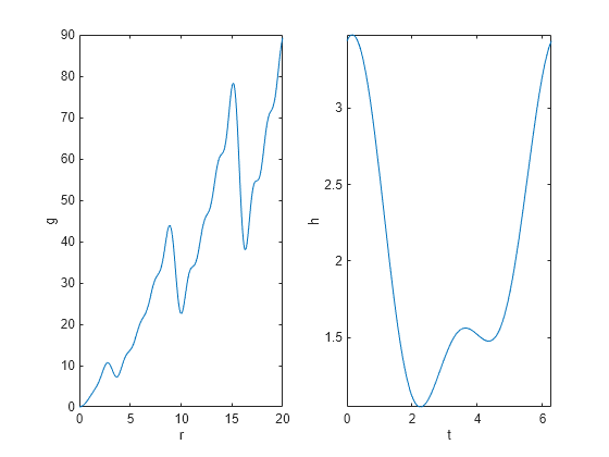
Figure contains 2 axes objects. Axes object 1 with xlabel r, ylabel g contains an object of type functionline. Axes object 2 with xlabel t, ylabel h contains an object of type functionline.

figure
fsurf(@(x,y) sawtoothxy(x,y), [-20 20])
% sawtoothxy is defined in the first step below
xlabel('x'); ylabel('y'); title('sawtoothxy(x,y)');
view(-18,52)

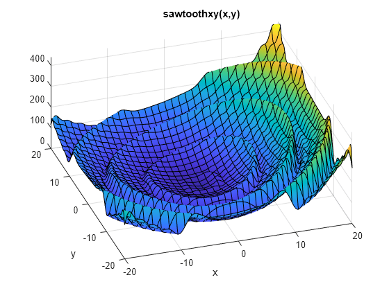
Figure contains an axes object. The axes object with title sawtoothxy(x,y), xlabel x, ylabel y contains an object of type functionsurface.

Le minimum global est à $r = 0$ , avec la fonction objectif 0. La fonction $g (r)$ croît approximativement linéairement dans $r$ , avec une forme en dents de scie répétitive. La fonction $h (t)$ possède deux minima locaux, dont l'un est global.

Le fichier sawtoothxy.m convertit les coordonnées cartésiennes en coordonnées polaires, puis calcule la valeur en coordonnées polaires.

type sawtoothxy

function f = sawtoothxy(x,y)
[t r] = cart2pol(x,y); % change to polar coordinates
h = cos(2*t - 1/2)/2 + cos(t) + 2;
g = (sin(r) - sin(2*r)/2 + sin(3*r)/3 - sin(4*r)/4 + 4) ...
    .*r.^2./(r+1);
f = g.*h;
end

Minimum global unique via `GlobalSearch`

Pour rechercher le minimum global à l’aide de GlobalSearch, créez d’abord une structure de problème. Utilisez l'algorithme 'sqp' pour fmincon,

problem = createOptimProblem('fmincon',...
    'objective',@(x)sawtoothxy(x(1),x(2)),...
    'x0',[100,-50],'options',...
    optimoptions(@fmincon,'Algorithm','sqp','Display','off'));

Le point de départ est [100,-50] au lieu de [0,0] donc GlobalSearch ne démarre pas à la solution globale.

Validez la structure du problème en exécutant fmincon.

[x,fval] = fmincon(problem)

x = 1×2

   45.7236 -107.6515

fval = 
555.5820

Créez l'objet GlobalSearch et définissez l'affichage itératif.

gs = GlobalSearch('Display','iter');

Pour la reproductibilité, définissez la valeur seed du générateur de nombres aléatoires.

rng(14,'twister')

Exécutez le solveur.

[x,fval] = run(gs,problem)

 Num Pts                 Best       Current    Threshold        Local        Local                 
Analyzed  F-count        f(x)       Penalty      Penalty         f(x)     exitflag        Procedure
       0      200       555.6                                   555.6            0    Initial Point
     200     1463   1.547e-15                               1.547e-15            1    Stage 1 Local
     300     1564   1.547e-15     5.858e+04        1.074                              Stage 2 Search
     400     1664   1.547e-15      1.84e+05         4.16                              Stage 2 Search
     500     1764   1.547e-15     2.683e+04        11.84                              Stage 2 Search
     600     1864   1.547e-15     1.122e+04        30.95                              Stage 2 Search
     700     1964   1.547e-15     1.353e+04        65.25                              Stage 2 Search
     800     2064   1.547e-15     6.249e+04        163.8                              Stage 2 Search
     900     2164   1.547e-15     4.119e+04        409.2                              Stage 2 Search
     950     2359   1.547e-15           477        589.7          387            2    Stage 2 Local
     952     2423   1.547e-15         368.4          477        250.7            2    Stage 2 Local
    1000     2471   1.547e-15     4.031e+04        530.9                              Stage 2 Search

GlobalSearch stopped because it analyzed all the trial points.

3 out of 4 local solver runs converged with a positive local solver exit flag.

x = 1×2
10^-7 ×

    0.0414    0.1298

fval = 
1.5467e-15

Le solveur trouve trois minima locaux, y compris le minimum global proche de [0,0].

Plusieurs minima locaux via `MultiStart`

Pour rechercher plusieurs minima à l’aide de MultiStart, créez d’abord une structure de problème. Comme le problème n'est pas contraint, utilisez le solveur fminunc. Définissez les options pour ne pas afficher d'affichage sur la ligne de commande.

problem = createOptimProblem('fminunc',...
    'objective',@(x)sawtoothxy(x(1),x(2)),...
    'x0',[100,-50],'options',...
    optimoptions(@fminunc,'Display','off'));

Validez la structure du problème en l’exécutant.

[x,fval] = fminunc(problem)

x = 1×2

    8.4420 -110.2602

fval = 
435.2573

Créez un objet MultiStart par défaut.

ms = MultiStart;

Exécutez le solveur pendant 50 itérations, en enregistrant les minima locaux.

rng(1) % For reproducibility
[x,fval,eflag,output,manymins] = run(ms,problem,50)

MultiStart completed some of the runs from the start points. 

10 out of 50 local solver runs converged with a positive local solver exitflag.

x = 1×2

  -73.8348 -197.7810

fval = 
766.8260

eflag = 
2

output = struct with fields:
                funcCount: 8574
         localSolverTotal: 50
       localSolverSuccess: 10
    localSolverIncomplete: 40
    localSolverNoSolution: 0
                  message: 'MultiStart completed some of the runs from the start points. ...'

manymins=1×10 GlobalOptimSolution array with properties:
    X
    Fval
    Exitflag
    Output
    X0

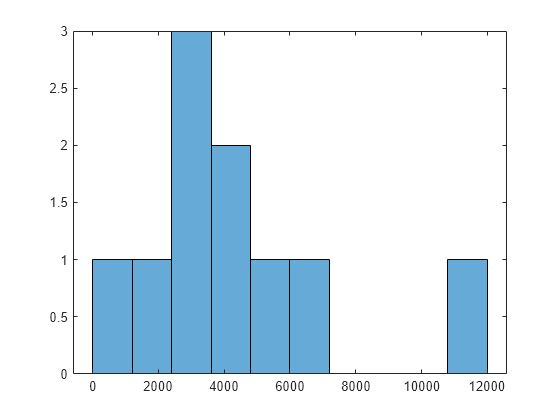
Le solveur ne trouve pas le minimum global près de [0,0]. Le solveur trouve 10 minima locaux distincts.

Tracez les valeurs de la fonction aux minima locaux :

histogram([manymins.Fval],10)

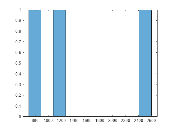
Figure contains an axes object. The axes object contains an object of type histogram.

Tracez les valeurs de la fonction aux trois meilleurs points :

bestf = [manymins.Fval];
histogram(bestf(1:3),10)

Figure contains an axes object. The axes object contains an object of type histogram.

MultiStart démarre fminunc à partir de points de départ avec des composants uniformément répartis entre –1000 et 1000. fminunc reste souvent bloqué dans l'un des nombreux minima locaux. fminunc dépasse sa limite d'itération ou sa limite d'évaluation de fonction 40 fois.

Voir aussi

GlobalSearch | MultiStart | createOptimProblem

Trouver des minima globaux ou locaux multiples

Minimum global unique via GlobalSearch

Plusieurs minima locaux via MultiStart

Voir aussi

Rubriques

Minimum global unique via `GlobalSearch`

Plusieurs minima locaux via `MultiStart`